Module 9 - Advanced Software Features

System Status, Communications & Logs

System Information

The system information tab displays details relating to important components that make up the system. For example, the Linux version or how long is left on the licence.

To access this window, select About from the System tab on the toolbar.

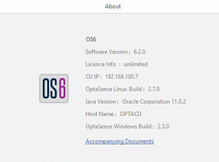
Figure 1: Left: Accessing System information / Right: System Overview Page

Selecting the Accompanying Documents link (above, right image) will open the supporting manuals for the software.

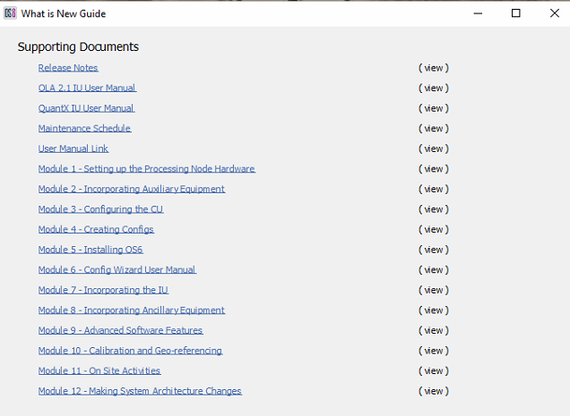
Figure 2: Supporting OS6 Manuals

System Health & Process Management

System Health

System Health provides the health state of the major processes and interfaces running on the system. To access this window, select System Health from the Process Management tab on the toolbar.

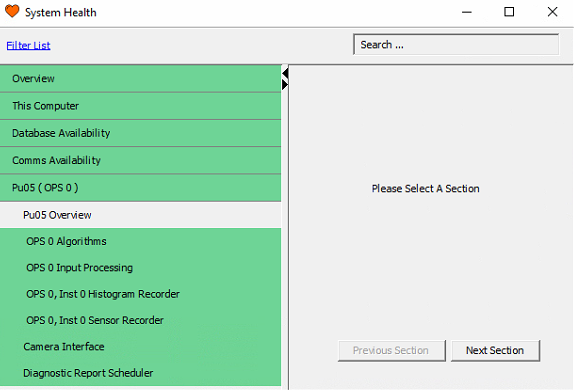
Figure 3: System Health

Processes that are running without issue will be highlighted in green; Processes that have been intentionally disabled will be highlighted in grey; And any processes that are in an error state will be highlighted red. A user notification will occur if a process enters an error state. In Figure 4, the histogram recorder can be seen to have entered an error state as a result of the Algorithms process being stopped.

The user notification can be expanded to provide further details about why an error has occurred.

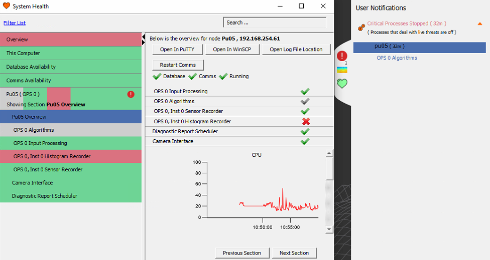
Figure 4: Process / Interface State / User Notifications

Stopping, Starting Processes

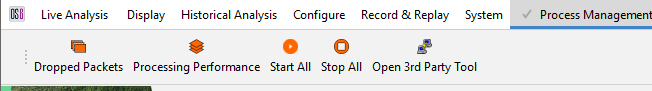
One way to stop/start all processes is to use the 'Start All' and 'Stop All' buttons under the Performance Management menu on the Overview display.

Another way to stop/start processes is to do this on a per node basis. This can be achieved by opening the System Health display and selecting a node. On this node, all processes can be stopped/started with one switch or processes can be stopped/started individually. Figure 5 showcases the ways processes can be turned off and on from System Health.

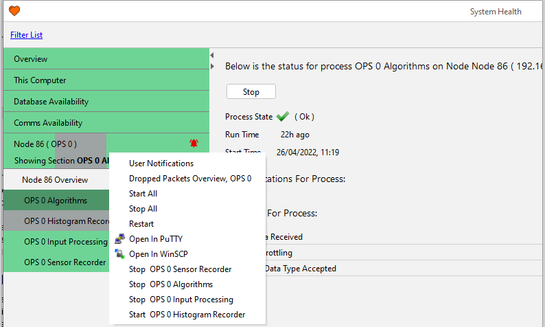
Figure 5: Stop / Start Processes / Interfaces

Node Status Overview

The status overview page displays each processing server (Node) and the status of the processes running on it. To reveal these, click on the required node. Each process can be stopped and restarted in two ways. 1. Right-click on the process and select Stop / Start. 2. Select the process, then Stop / Start from the central window.

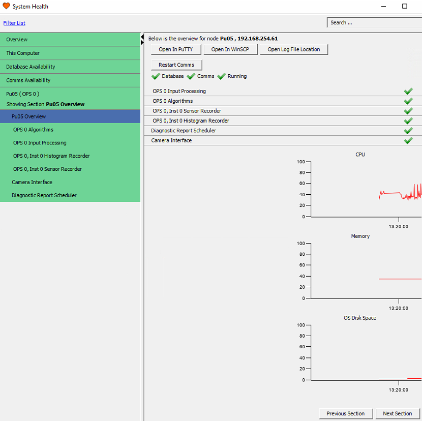
Figure 6: Processing Node Status Overview

Restart Processes Button Overview

Notice the buttons above. Clicking on them will open the corresponding 3rd party tool on the CU.

1. Open in PuTTY - Utility that provides console access to Linux on the node.
2. Open in WinSCP - Utility that provides Linux GUI folder and file navigation on the node.
3. View Log Browser - Displays GUI logs of the node.
4. Restart Comms - Restarts Hazelcast on the node.

Database Availability

This section details the connection state of the database distributed on a prescribed number of nodes (processing units and dual processing units) on the system. The database view can be expanded or closed by left-clicking on the Database banner. This section is for information purposes only and gives a system overview of the database connections. To access this function, from the toolbar, select Process Management and then System Health.

Figure 7: Expanded Database Availability view

Comms Availability

The first section details the connection state of all nodes (processing units and dual processing units) on the system. The system communication view can be expanded or closed by left-clicking on the system communications banner.

Figure 8: Expanded System Comms Availability view

Global Process Management

Global Process Management enables the user to stop and start important processes collectively across the system. The following list describes those processes.

Restart Processes Button Overview

1. Stop / Start All – Restarts all-important processes listed in the System Health.
2. Stop / Start Algorithms – Restarts detector algorithm processes.
3. Stop / Start Input Processing – Restarts the data stream process from the IUs to the algorithms.
4. Stop / Start Sensor Recordings – Restarts the sensor recordings processes.
5. Stop / Start Histogram Recordings – Restarts the histogram recordings processes.
6. Restart Comms Cluster – Restarts the communication process across all nodes.

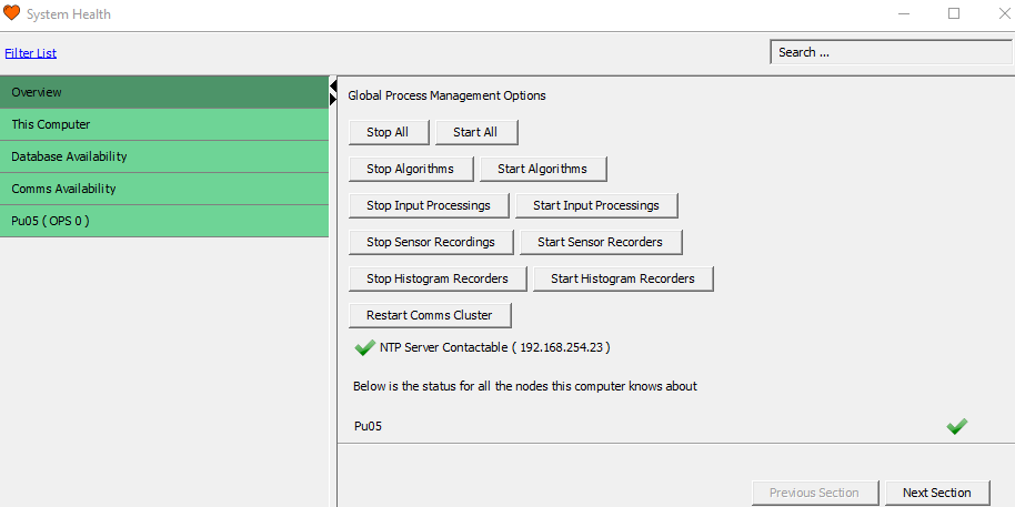
Figure 9: Global Process Management

Dropped Packet

Dropped Packets are an indication that the system is unable to keep up with the data being received. When this happens, an error will appear in the User Notification window. Some examples of causes of drop packets are having too many detectors running simultaneously or if a hard drive is running slowly. If dropped packets are occurring regularly, an investigation into the cause must be undertaken.

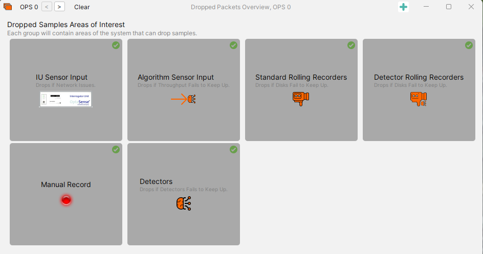
Figure 10: Clearing Dropped Packets

Processing Chain Performance

Processing Chain Performance gives a resource overview of all processes running on the system. To access this window, select Processing Performance from the Process Management tab on the toolbar. Values includes:

• The amount of time spent in each processing step
• The current and max watermark levels seen in each of the buffers
• The number of packets that have been lost within a given step

High values can indicate processing strain and packet losses should be investigated.

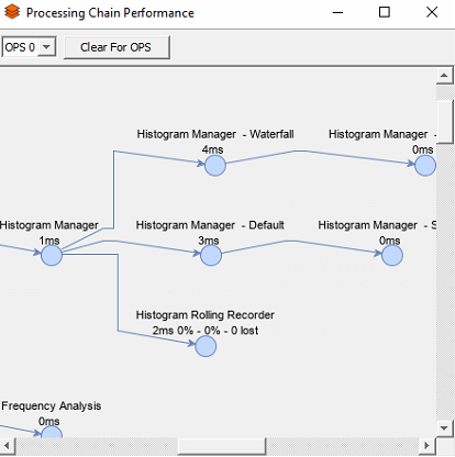
Figure 11: Processing Chain Performance

Historical Analysis

Diagnostics Report

This feature enables the user to generate a health diagnostics report, either manually or automatically, which can be stored on the CU or sent to an email recipient. To access this window, from the toolbar, select Historical Analysis and then Diagnostic Reports.

Figure 12: Diagnostic Reports

Generate a New Manual Report enables the user to compile a report based on the health of the system at a given date. View System Generated Reports enable recall of previously system generated reports. These can be searched for by selecting a pre-set time range or selecting the dates manually.

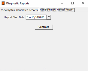
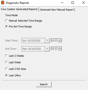
Figure 13: Left – New / Right - Report Existing Report

Exporting Report

Having selected Generate, shown in the left image above, the report can be exported to a chosen location on the CU Having clicked save, the report will take at least a minute to compile.

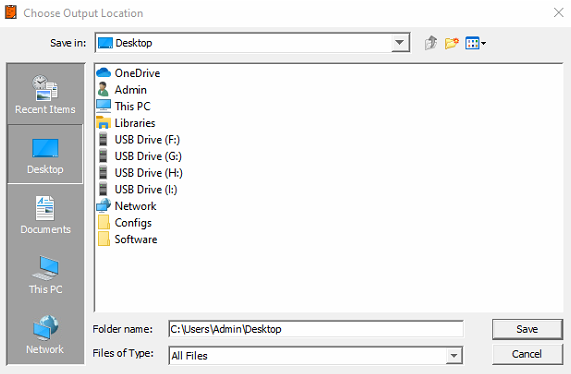
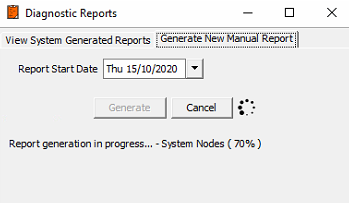
Figure 14: Left – Selecting Storage Location / Right – Report Compiling

Once the report is complete, it will be stored in the chosen location and it will automatically open in the CU's internet browser.

Diagnostics Report Scheduler

Diagnostic Report Scheduler enables the user to set the software to periodically generate system health diagnostic reports. To access the scheduler, from the toolbar, select Configure, Wizard and then Diagnostic Report Scheduler

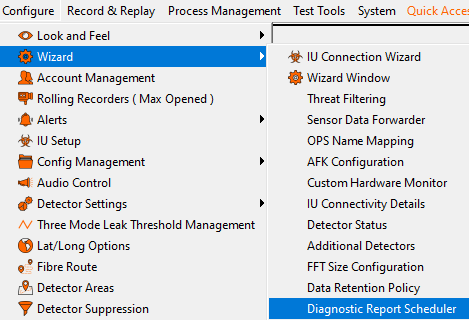
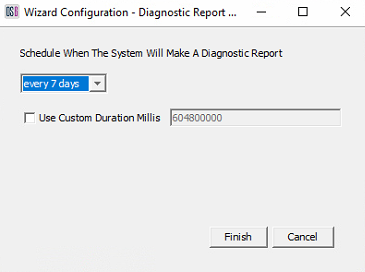
Figure 15: Left – Navigate to Scheduler Right – Setting Report Generation Period

Reviewing Diagnostic Reports

Diagnostic reports can be opened and viewed in an internet browser.

System Overview and its features can be seen highlighted above.

• System Overview - Provides details on the number of nodes within the system, the total fibre length coverage and the current version of software the system is running on.

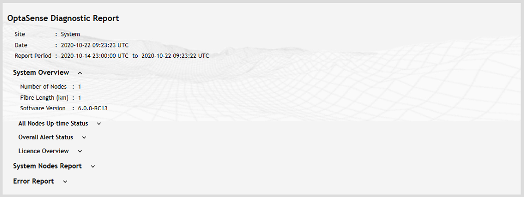
Figure 16: Front Page Display

All Nodes Up-time Status

Reports how long the nodes have been running and what errors occurred. Note with multiple nodes, more horizontal bars will appear in the chart below. Hover over the required node to display its information.

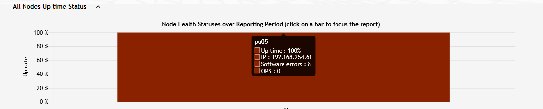
Figure 17: All Nodes Up-time Status Display

Overall Alert Status

Provides a colour-coded bar graph displaying the levels of alerts (high, medium and low) on each OPS during the reporting period. The same chart can be displayed for the medium and low alert count.

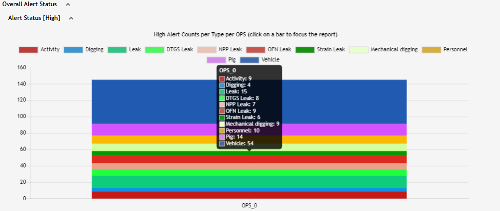
Figure 18: Alert Status - High

Licence Overview

Gives details regarding the licence applied to the system.

Figure 19: Licence Overview

System Node Report

Provides an overview of the following aspects. Note, select the required node via the Select Node drop-down arrow.

• Number of alerts,
• Node uptime.
• Overall node CPU, memory and disk usage

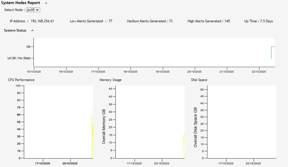
Figure 20: System Status

Software Processes

Displays the health of main software processes and how long they've been running. The graphs on the right provide a visual overview of the strain put on the hardware resources.

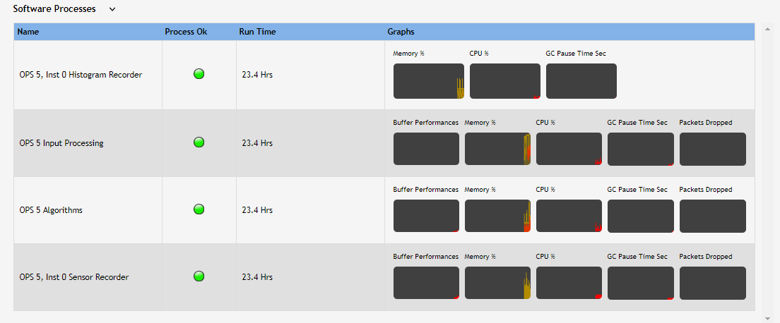
Figure 21: Software Processes

Software errors

Displays fatal error messages.

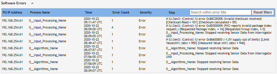
Figure 22: Software Errors

OPSes Report

Provides information for the OPS/s connected to a node. This is dependent on whether a PU or DPU has been selected using the bar graph in the 'All Nodes Up-Time Status' section or using the drop-down box in 'System Nodes Report'. OPS ID, the number of channels, sampling rate, Interrogator IP address and channel length are all shown.

Figure 23: OPS Report

IU Connectivity Status

Displays IU has connection time and any dropouts.

Figure 24: IU Connectivity Status

The Alert Information Heatmap

Displays the frequency of high alerts across all channels on an OPS. A slider is provided to change the colour graduation of frequency groups of alerts; this allows the user to quickly identify the channels where 'hot spots' of alerts are being raised. The mouse scroll wheel and left-click drag can be used to zoom into the chart and pan left or right.

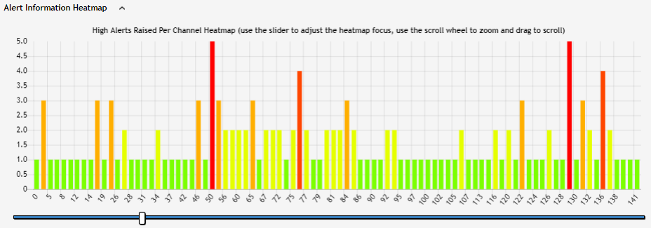
Figure 25: Alert Information Heatmap Display

Alert Count by Type

Display alerts (high, medium & low) by type and number of occurrences during the reporting period.

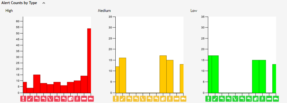
Figure 26: Alert Information Heatmap Display

Error Report

Provides the user with all system messages (info, warning, fatal and error). The list can be filtered using the search within the error title box and sorted by each column by clicking on the column title. Reset filters reset any manipulation carried out on the table.

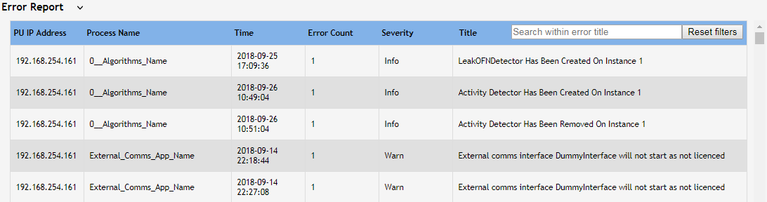
Figure 27: Error Report Display

Historic Waterfall Data

The alert history waterfall enables the visualisation of historic data. To access it from the toolbar, select the Alert History Waterfall button from the Historical Analysis tab.

Figure 28: Historical Waterfall Data

The dialog box shown in Figure 29 will appear where the desired OPS, date/time and channel range can be specified. The data source can also be changed to retrieve data from other rolling recorders. The search function is limited to a 24 hours period.

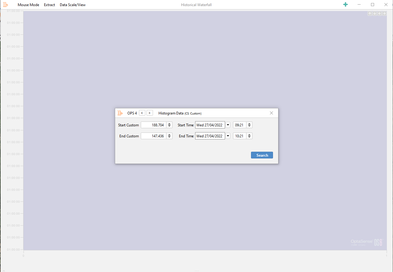
Figure 29: Selecting data based on OPS, date/time & channel range

Assuming the data is available, a snapshot of the data and any associated alerts from within the time span will appear (Figure 30).

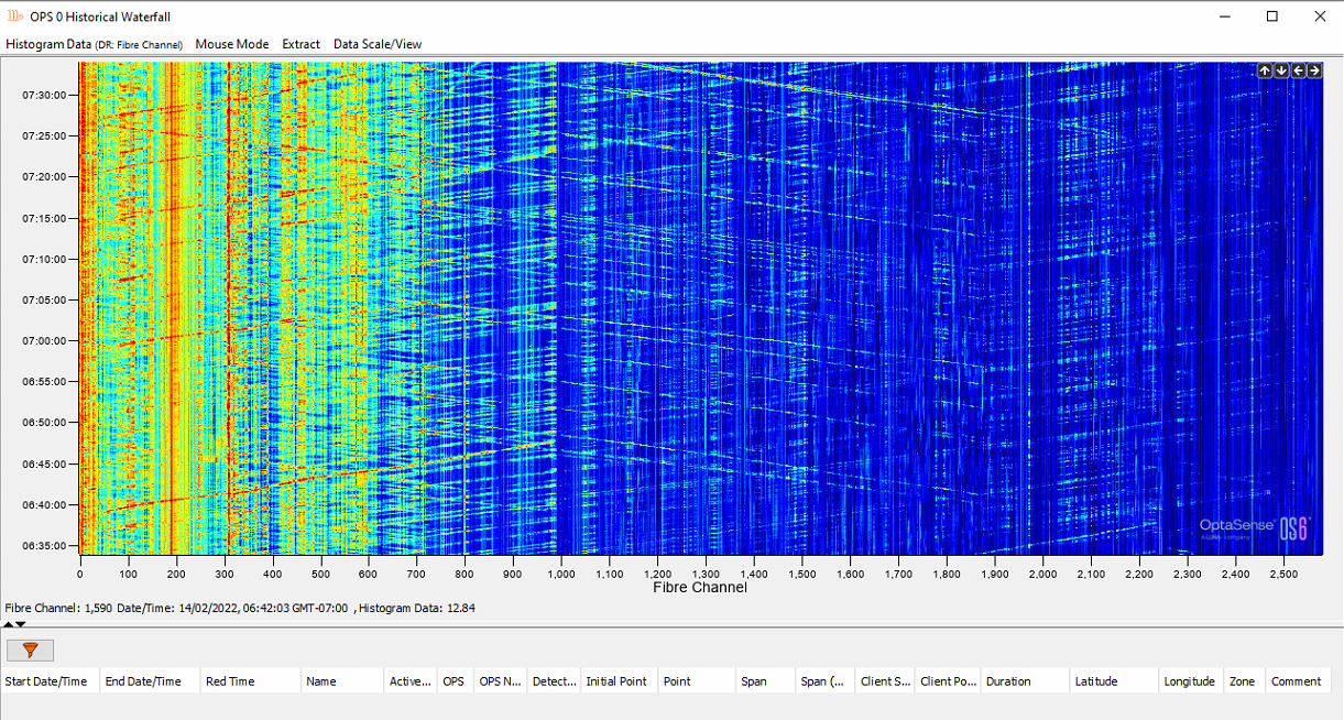
Figure 30: Historic Waterfall

Extracting Data

Data can be extracted from each of the rolling recorders as raw data or to CSV as required. Sensor data can require large amounts of space and the overall file size is limited.

Figure 31: Extracting Sensor Data

Name the data accordingly and choose between copying to Server's Record Location or Copy to CU. When copying to CU, the user will be prompted to choose a storage location.

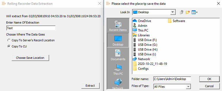
Figure 32: Choosing Storage Location

Copying to Server Record Location will store the data in the same directory as manual recordings. If using a Linux navigation utility, e.g. WinSCP, by default, the storage location is /mnt/disk4/ManualRecord0

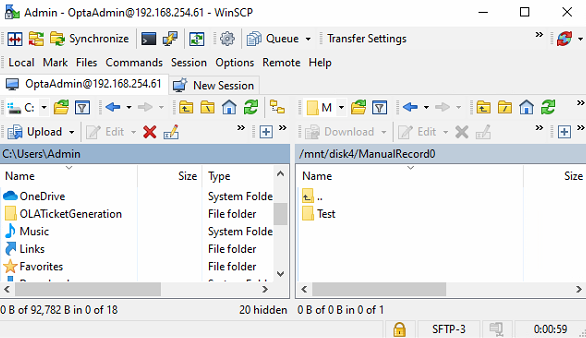
Figure 33: Linux Navigation Utility

Historical Multi-Channel Trending

The historical multi-channel analysis tool enables the user to plot histogram and leak data recorded on the system at a given date/time.

There are 2 ways this feature can be accessed.

1. From the toolbar, select Historical Analysis, then Historical Multi-Channel Trending.
2. On the OS main window, select the alert list icon (high, medium/low). Now click the required alert, right-click and select Historical Multi-Channel Trending.

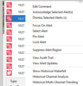
Figure 34: Left - Historical Multi-Channel Analysis / Right - Selecting the Feature from Alert

In the window below, a line graph is plotted outlining the source of data from an alert. To manually choose a source, click Add Source. Scale Options enable the time of the source to be edited. The + button enables another source to be plotted within the same window. The x button removes a source.

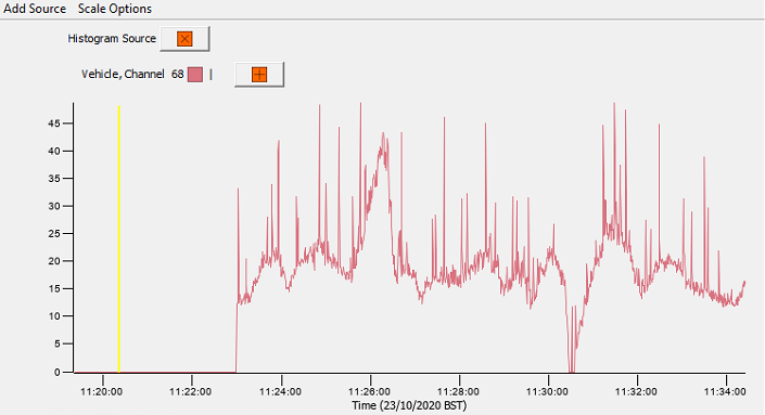
Figure 35: Analysis Options

Historical Alerts

Historical alerts can be displayed. These alerts can then be exported into a chart or CSV format. To access this feature, from the toolbar, select Historical Analysis and then Historical Alerts.

Figure 36: Analysis Options

From the toolbar on the left side, the user can select the duration they require to run the report on. The user can also select the level of alert (low, medium or high), a specific alert type and span the search over multiple OPS. Once this form is filled out, users can either extract the results to CSV/HTML or display the results on the right-hand pane showing all information stored about the occurrences, e.g. start and end channel, type (personnel, vehicle etc.), latitude and longitude and comments entered by the user. This right-hand pane uses a 'Page' mechanism in that users can page through 10000 alerts at a time.

Note the alerts highlighted with colour indicate they haven't been acknowledged by the user.

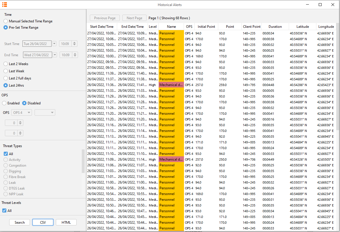
Figure 37: Historical Alert List

Historical Alert Extraction

There are two options for exporting alert data.

The button will export alert data into Microsoft (MS.) Excel file format. Once the button is clicked, a prompt will ask you to confirm the export; select yes. Choose the desired location and click save. Another prompt will appear confirming that the export has finished.

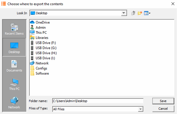
Figure 38: Exporting Alert Search to MS Excel

The button will export the data into web page format. Once the button is clicked, choose the desired location, and select Open. Now select the required charts from the chart option drop-down box or select Add All. Select Generate to compile the report.

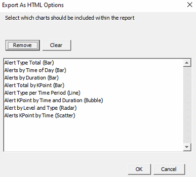
Figure 39: Exporting Alert Search Query to HTML

Once the report has finished, the following prompt will display.

Figure 40: Confirmation of Successful Report Generated

The contents of the zipped file will need to be extracted to view its contents.

Figure 41: Unzipping Report to Run in Browser

Once extracted, navigate to the AlertReport.html file. Right-click on it and open it with a web browser.

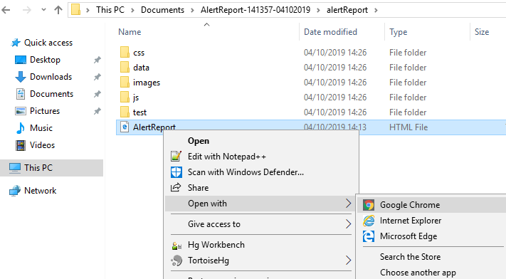
Figure 42: Opening Report in Browser

Alert Charts

There are three tabs on the top left of the browser.

• Charts - Displays a list of charts
• Waterfall - Provides a histogram waterfall based on the duration selected in the alert search query.
• View - Selecting Default will change the view mode to extended. This provides increased viewing focus on charts. Theme: Changes the white borders of the webpage to grey.

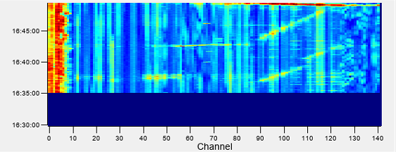
Figure 43: Charts that can be Selected

Chart Types

Alert Type Total (Bar)

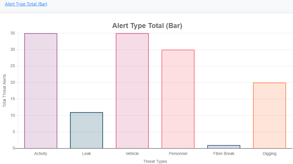
Figure 44: Alert Type Total

Alerts by Time of Day (Bar)

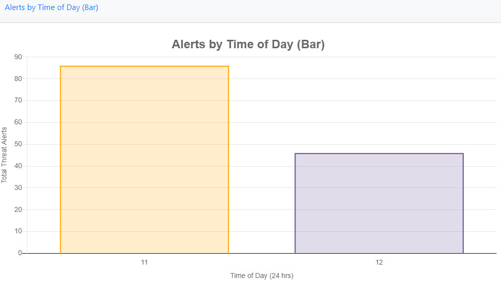
Figure 45: Alerts by Time of Day

Alerts by Duration (Bar)

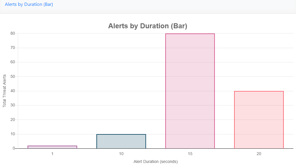
Figure 46: Alerts by Duration

Alert Total by KPoint (Bar)

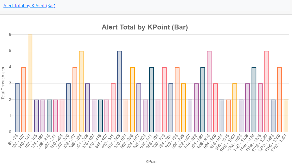
Figure 47: Alert Total by Kpoint

Alert Type per Time Period (Line)

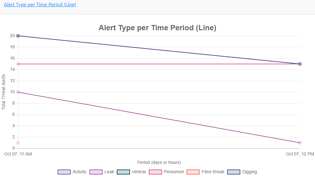
Figure 48: Alert Type per Time Period

Alert KPoint by Time and Duration (Bubble)

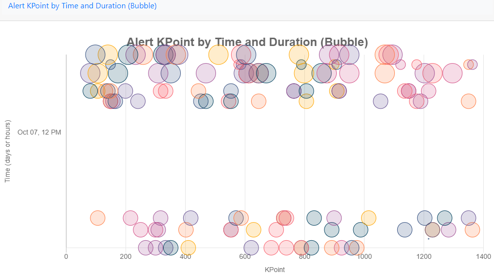
Figure 49: Alert KPoint by Time and Duration

Alert by Level and Type (Radar)

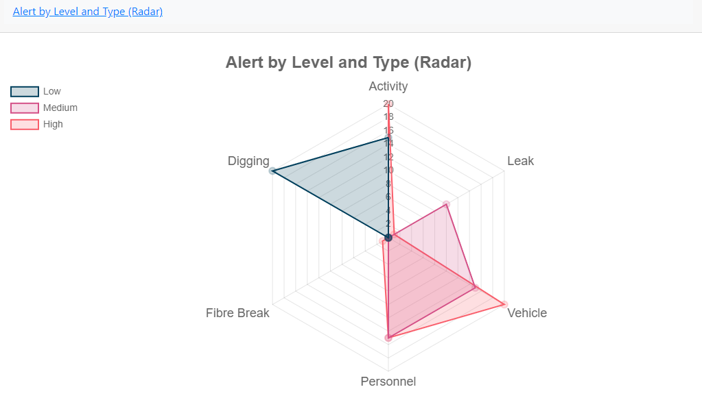
Figure 50: Alert by Level and Type

Alerts KPoint by Time (Scatter)

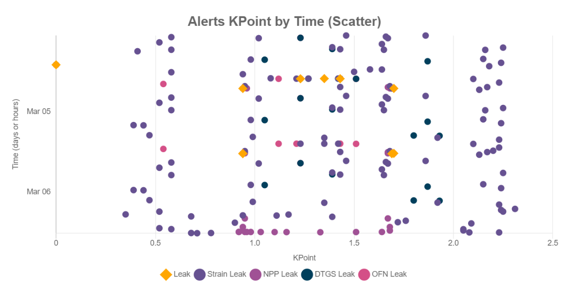
Figure 51: Alerts KPoint by Time (Scatter)

Log Event Viewer

The log event viewer enables the user to recall any System errors/warning etc that have occurred. To access this feature, from the toolbar select Historical Analysis and then Log Event Viewer.

Figure 52: Log Event Viewer

From the toolbar on the left, the user can select the duration they require to run the report on. The user can also select the level of the logs (unhandled, fatal, warning or debug errors). Once the Search button is selected, the logs will appear in the right pane showing all information stored about the log occurrences. Once the report has been generated, the user can extract the report to a text file.

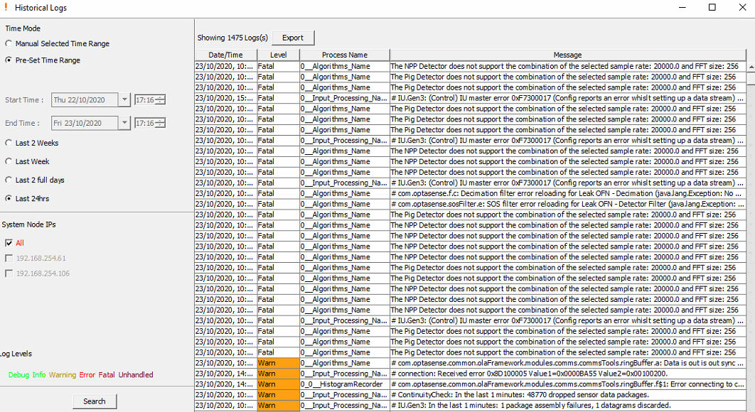
Figure 53: Log Event List

Auditing

Auditing enables the user to view the changes made to the system and by whom. To access this feature, from the toolbar, select Historical Analysis and then Audits.

Figure 54: Audits

From the toolbar on the left the user can select the duration they require to run the audit on. By default, all nodes, actions and by whom they were made by will be selected.

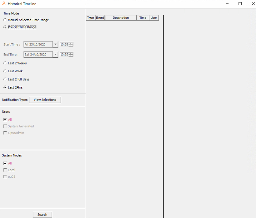
Figure 55: Auditing search dialog

To change what actions are to be listed, select View Selection as shown in the image above. Uncheck the unrequired actions.

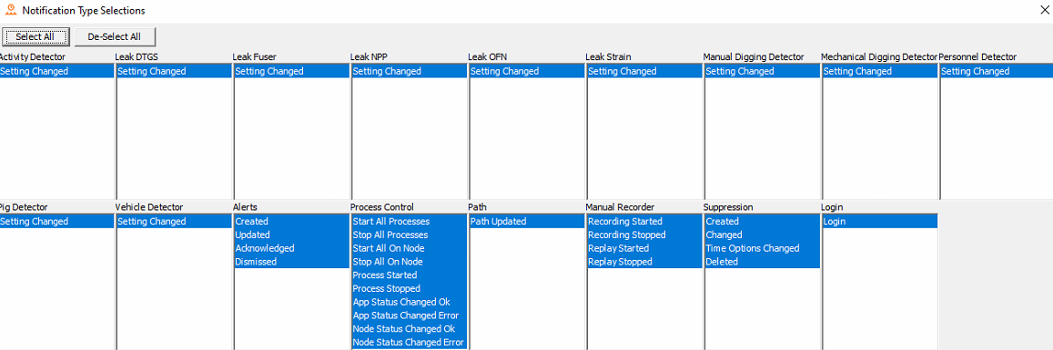
Figure 56: Audit Viewer

Select search to run the audit. To display more information on an instance, hover over. To quick filter, use the search box and type the name of action / user required. The column headers can also be used to filter. For example, selecting type will order the list of actions by the type of instance.

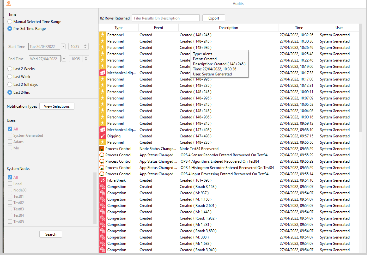
Figure 57: Audits List

- Audit Trail

Along with seeing audits in the format seen in Figure 57, audit trails/linked audits can also be viewed. Audits that are linked normally share a characteristic like an identifier or name so that the change history for that link can be seen overtime. An example of this is viewing an alerts' audit trail overtime to see when it was created, updated, or acknowledged etc or to see the change history of a Detector setting.

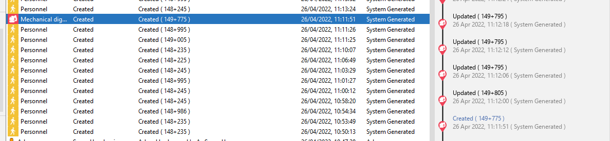
Figure 58: Audit Trail for an audit in the Audit Window

The first way to view a trail for an event is to use the Auditing Window as seen in Figure 57. In this display, when a row is selected, the audit trail for that row is shown to the right with the selected row in that trail highlighted in blue.

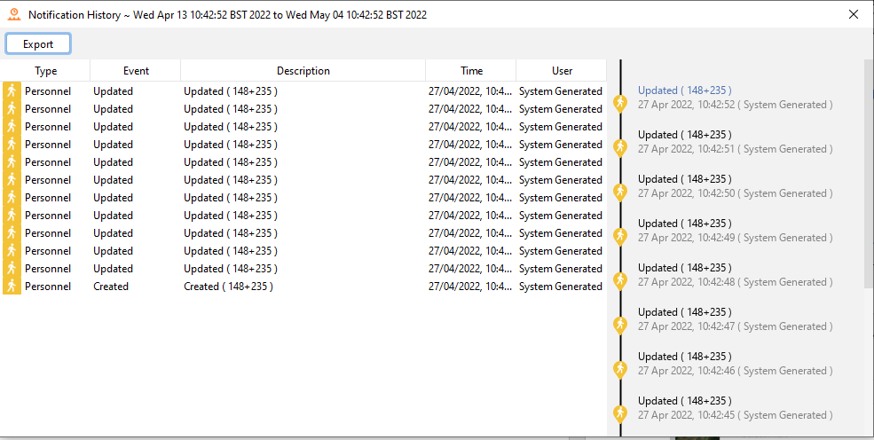
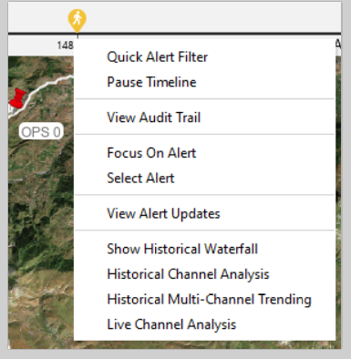
Figure 59: Audit Trail for an audit in the Audit Trail Window

The second way to view the trail for an event is to use 'View Audit Trail' menu seen on the Live Timeline Menu and Alert menu (Totes, Map etc). This option will open a display in which the audit trail will show for the selected event. This display will list the audit trail in table form and in a format like Figure 58. This display also allows the trail to be exported to csv.

Historical Process Metrics

Process report charting enables the user to select the resources that they want to monitor. Resources that can be monitored include:

Memory (%) – Displays the memory usage for the specified process. The yellow area displays the percentage of memory currently allocated to the process as a percentage of the maximum permitted. The red line shows the current memory usage. The most important feature of this chart is the lowest reached by the red line. This reflects the amount of memory in use by the process that is in long term use.

CPU (%) - CPU usage for the specified process. The total CPU usage will be made up of the load on each process combined (plus operating system processes).

GC Throughput (%) - Amount of time being spent in the Java garbage collector as opposed to time spent running process code. Consistent drops more than a few percent below 100% should be investigated.

GC Pause Time Sec – Time spent by the Java garbage collector freeing temporary memory. The more time spent here, the less time being spent by the CPU running process code. Occasional pauses of one or two seconds are acceptable but long pauses are likely to cause issues.

IU Temperatures Celsius – Temperature readouts from within the IU

To access this feature, from the toolbar select Historical Analysis and then Historical Process Metric.

Figure 60: Historical Process Metric

From the toolbar on the left the user must select the required node, monitoring period and what processed are to be displayed as plotted charts. It's advised that continuing spikes, dips, or absent periods be investigated.

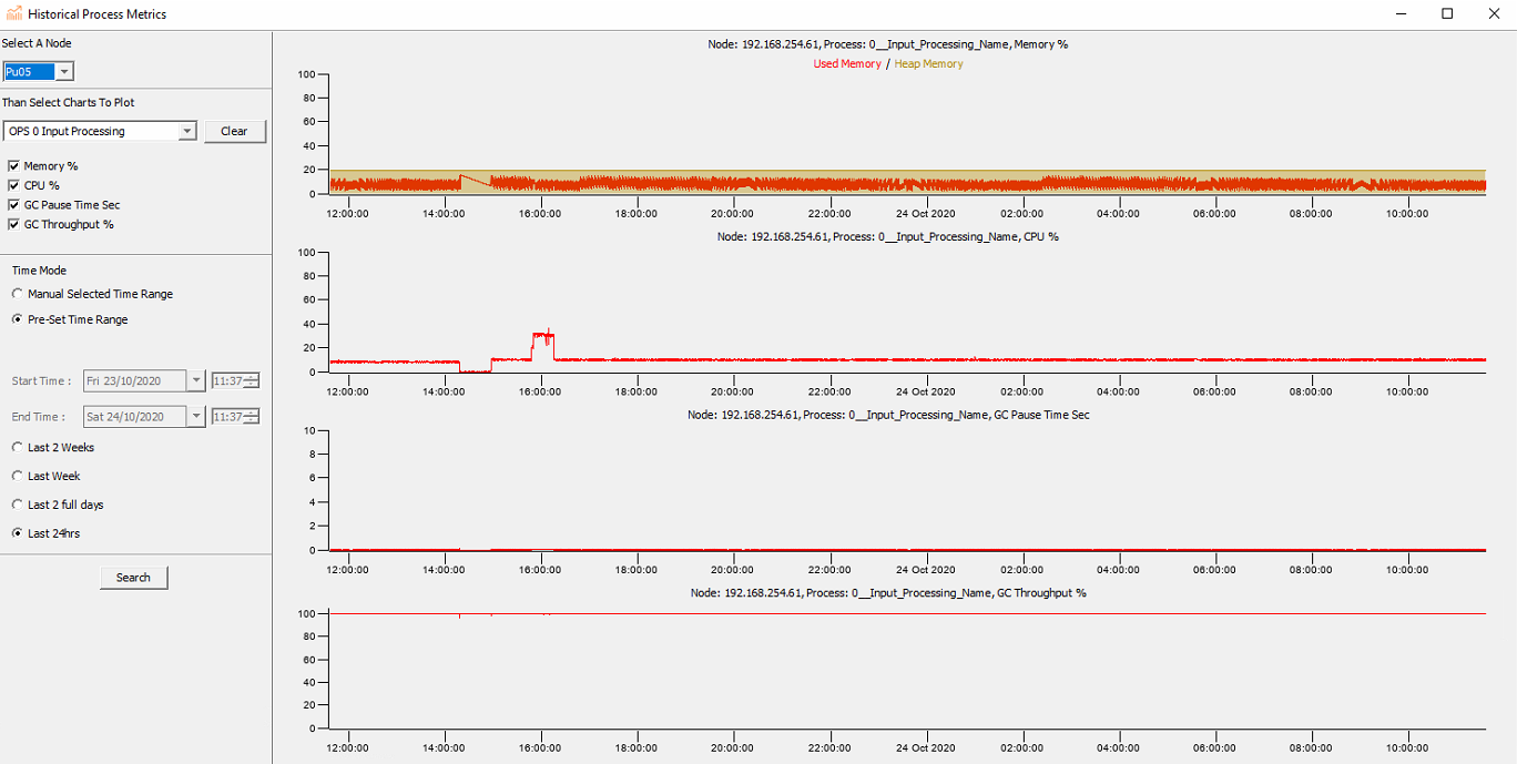
Figure 61: Process Report Charting

Rolling Recorders

The Rolling Recorders section in the configure tab allows the operator to configure the rolling recorders for the histogram, sensor data, and leak algorithms (Error! Reference source not found.).

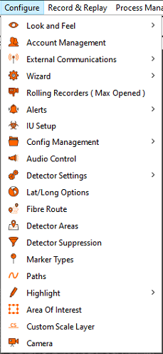
Figure 62: Configure Menu with Rolling Recorder Visible

The rolling recorder configuration window (Figure 63) will show the disk(s) associated to the selected node and show disk allocation associated to each data stream associated to the rolling recorder. The rolling recorder path is set automatically and default settings for storage can be applied per OPS or globally across all nodes.

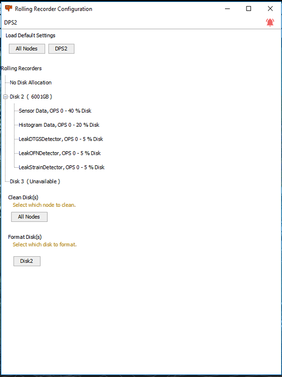
Figure 63: Rolling Recorder Configuration Screen

It is possible to change storage allocation to each stream by right clicking a stream and adjusting the allocated storage space, shown as a percentage of the available space on the rolling recorder drive (Figure 64).

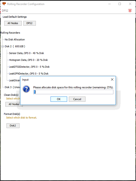
Figure 64: Rolling Recorder Storage Allocation

Config Management

The Config Management option in the Configure tab (Figure 65) allows for import and export of config files and folders within the operator software (briefly covered in Module 4: Config Creator).

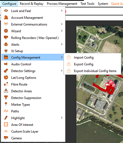
Figure 65: Configure Menu with Config Management Expanded

Import Config allows for the import of either an entire config folder (Figure 67) or import of individual config files (Figure 66).

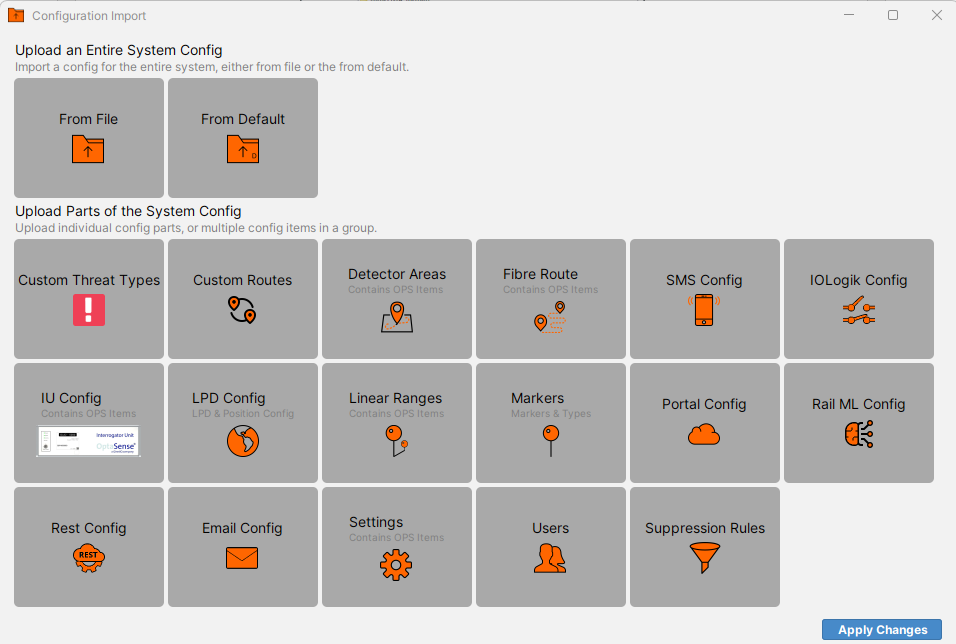
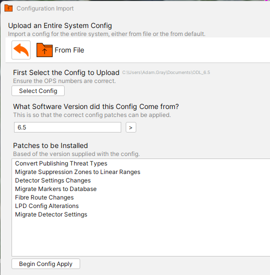
Figure 66: Import Config Figure 67: Import Config From File

Export Config allows for the export the entire config folder to a target location on the CU (Figure 68).

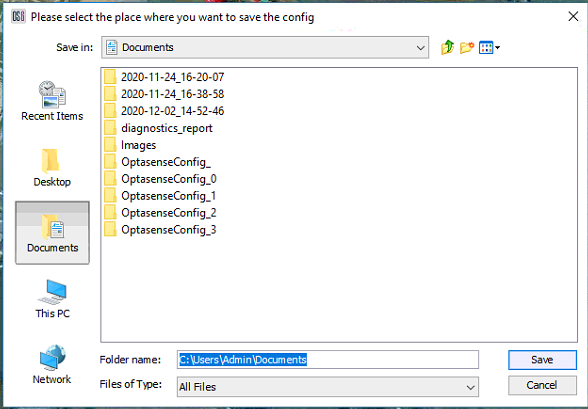
Figure 68: Export Config

Export Individual Config Items allows for the export of individual items from a config, following the logic of import of individual config files, the orange arrows allow for the menus to be expanded or collapsed (Figure 69).

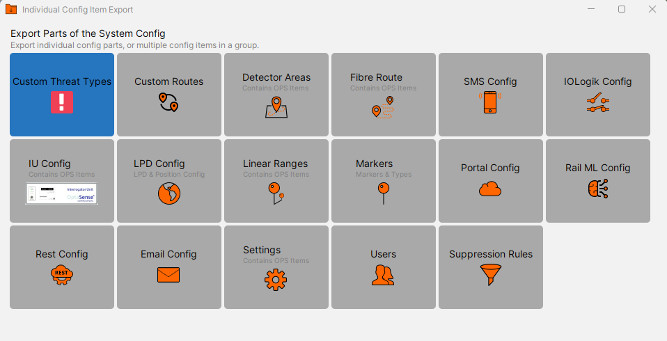
Figure 69: Export Individual Config Items

warning

Config files should only be changed by an expert user or after consultation with OptaSense Support. Changes to files may require additional user action to utilise the desired changes and uncontrolled changes may be damaging to the system.

Manipulating Map Screen Artefacts

Fibre Layer

The Configure>Fibre Route panel enables the user to make changes to an existing fibre route. This feature is useful should the physical fibre change geographically or in terms of length.

To open the Fibre Layer Configuration panel, from the toolbar, select Configure and then Fibre Route (Error! Reference source not found. 70).

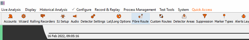
Figure 70: Accessing Fibre Route configuration

There are several options the user can use to aid when configuring of the fibre route.

Checking the options numbered below will show the following fibre route display overviews.

1. Nodes
2. Fibre Route – fibre route in line format
3. Channel Coverage
4. Calibration Points
5. OPS Names – Name of OPS covering a given section on the fibre route.
6. Other OPSes – Show all OPSes
7. Centre On Map Display view on chosen OPS
8. Fibre Color – Color of fibre route.
9. OPS Drop Down – Select specific OPS

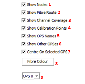
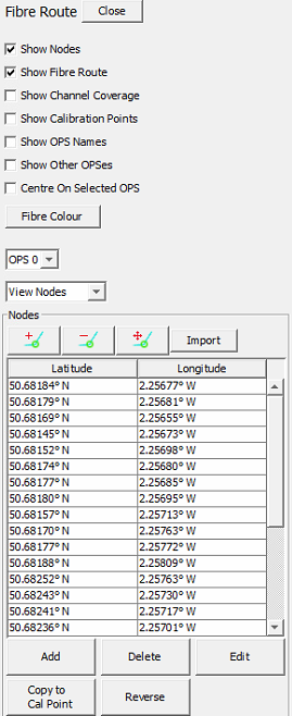
Figure 71: Fibre Route Visual Options

Examples of the more important options applied.

Show Nodes: Green circles mark the fibre route and generally denote a change of direction

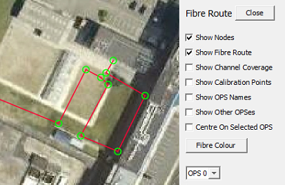
Figure 72: Showing Fibre Nodes

Show Channel Coverage: Blue circles denote the channel coverage selected. Should not overlap or have spaces between them

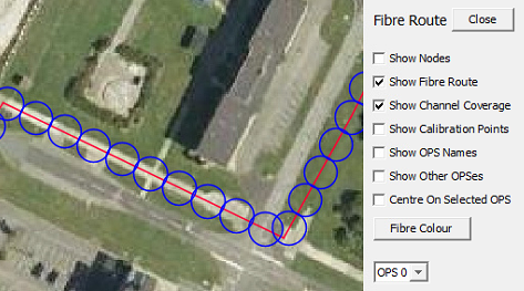
Figure 73: Showing Channel Coverage

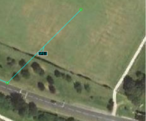
Show Calibration Points: Yellow crosses – used to refernce the fibre to the ground and contain position and optical distance information

Figure 74: Showing Calibration Points

1. Choose between fibre route node / cal points configuration
2. Node and calibration point edit buttons (map window)
3. Import fibre route – Refer to Module 4 Config Creator for more information regarding importing fibre routes
4. Copy to Cal Point – Takes a selected node point and creates a calibration point. (Note, when using, the user must switch to cal points and configure the additional information required to plot the point).
5. Add, delete, edit and reverse change node point.

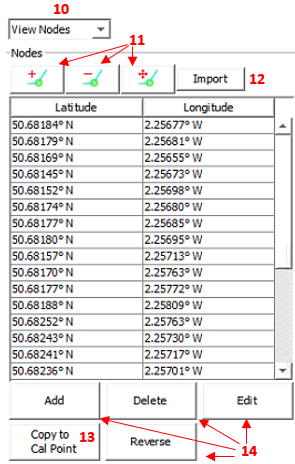
Figure 75: Fibre Route Edit Options

When switching to plotted calibration points, it's good to have a basic understanding of the following numbered points below.

1. Switch between displaying calibration points in terms of optical distance along fibre or in fibre channels
2. Toggle on and off calibration points. This is useful if the cal point was acting as a place holder.

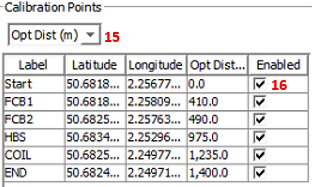
Figure 76: Calibration point Pointers

The user should regularly save their actions as they make changes the fibre configuration. It is advised to save every couple of actions. Should a mistake be made within those actions, the undo button can be used. The button below will appear after any change.

Figure 77: Calibration point Pointers

Nodes

Fibre nodes are generally provided by the client and are imported from a .csv file. Once the fibre layout has been added to the map layer there is usually no requirement to change it. In exceptional circumstances the fibre can be edited with the following buttons:

Clicking add node (ensure the button becomes shaded blue) and then any on the map will add a node at that point from end of the fibre (after the last node in the node list). A node can also be added anywhere along the fibre if the fibre route itself is clicked. Clicking the remove button followed by any node will remove that node. The fibre will automatically insert itself between the remaining nodes. Clicking move node will allow a node to be selected and 'dragged' to a new location. The fibre remains attached to the zone. The save or undo options become available after each action.

Figure 78: Node Configuration

Channel Coverage and Calibration Points

The channels are represented by blue circles that have the same diameter as the selected channel spacing. Geo-referencing is required to ensure that the length and route of the fibre that has been be placed onto the map layer is correct and accounts for loops of fibre that may be buried in splice chambers, etc. These loops can then be 'compressed' into a single channel enabling accurate alert posting to the map screen. The channel coverage circles are linked directly to the calibration points.

The calibration points contain data about the optical distance between each point as well as a unique name and geographical reference for placement. Right clicking on the desired calibration point will bring up the 'Edit Calibration Point' box. This is where the Optical Distance from the last calibration point can be changed and the Calibration point can be enabled or disabled.

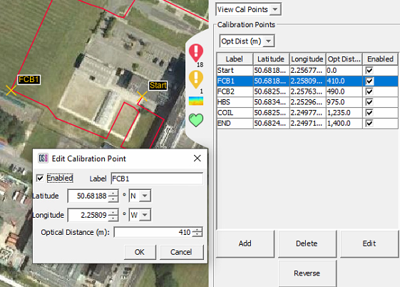
Figure 79: Calibration Point Editingclient

Custom Routes

Paths

Paths can be created on the Map screen to highlight features like roads, tracks, rivers and other geographical markers.

To begin creating a path, select Custom Routes from the Configure tab.

Figure 80: Custom Routes Location

Clicking 'Add' will load the add new custom route dialogue box up an Input box and prompt for a new for the new path. Ensure that the Route Type is set to "Path", enter a path name and click OK. The colour can be changed before selecting OK if desired.

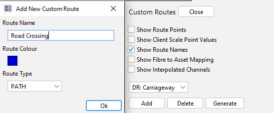
Figure 81: Path creation from custom routes

To start drawing a path, select the Add Route Nodes button in the custom routes dialogue and click on the map display where the first point is positioned. Select a second point, to which a line will be drawn. Additional points can be added between two existing nodes by creating a node close to the line between the two nodes. To remove a point, select the Remove Route Nodes button and click on the required point to delete it. Selecting the Move Route Nodes button allows existing nodes to be manipulated into a different position. Once the path is drawn, either add more custom routes as required or press Close. Pressing Close will open a Save changes prompt where changes can be saved or ignored. If adding multiple routes, it is advisable to save changes regularly.

Figure 82: Path on the map display

Asset Route

Asset route mapping allows the operators to create custom routes that can be used within detectors to address the differences between fibre route and asset routes – for instance, the effect of optical coils. Asset routes make use of a 'Fibre to Asset Mapping' algorithm to enable monitoring of an asset in relation to the monitored fibre. Notable examples where this would prove useful would be road and rail assets.

note

Only the Road Detector can currently make use of Asset Routes.**

To create an Asset Route, select configure custom routes from the toolbar and add a new route. Give the Asset Route a name and ensure that Asset Route is selected in the drop-down menu (Figure 83). An Asset Route will always be mapped to Fibre Channels.

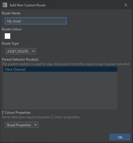
Figure 83: Asset Route Creation

Select OK to create the route. It is then possible to add/remove and move Asset points on the map from the asset dialogue. As shown in Figure 84, once an asset route has been created, if the Show Fibre to Asset checkbox is selected, the interpolated channel mapping to each asset channel is visible (denoted by the short blue lines).

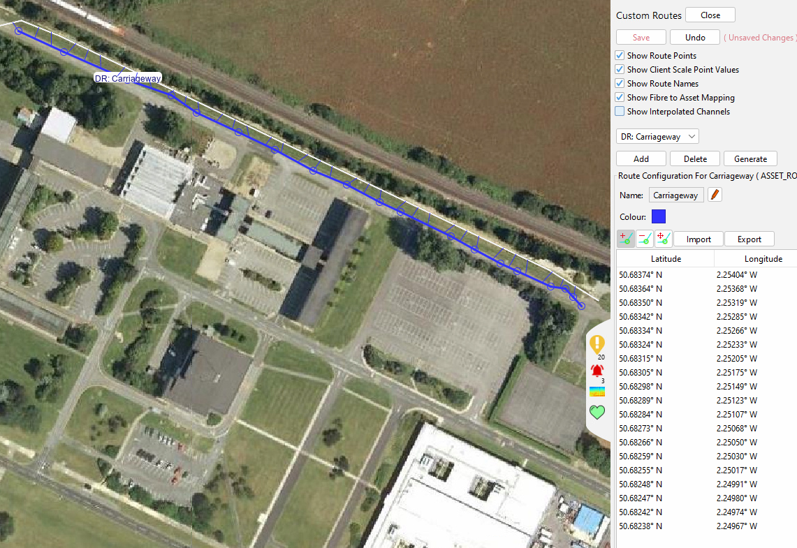
Figure 84: Asset Route showing mapping to OPS channels

tip

Assets can be grouped into ‘Detector Routes’ which consists of Fibre and Asset Routes

Client Scale

The client scale is used to plot a series of reference points along Detector Routes – most commonly K-points along pipelines. A client scale allows alerts to be output with custom markers that the client may be more familiar with. The client scale can also be used on the waterfall display to change the x-axis. When using a client scale on the waterfall display the x-axis will always run increase from left-to-right; The fibre channels will automatically be flipped if the scale runs in the reverse order to the fibre channels. While a Client Scale can span multiple OPS, the waterfall display will only display the section that is relevant to the currently selected OPS.

Utilising a 'Fiber to Asset Mapping' mechanism means it is now possible to create client scales that follow an asset (e.g. a pipeline) rather than the fibre route. This allows unnecessary fibre channels to be removed from the fibre route when displayed on the waterfall (for instance, optical coils or fibre around a block valve station). Multiple Client scales can be created to allow a waterfall to show just the relevant channels for different routes.

Adding a New Client Scale

To add a client scale, open the custom routes dialogue and choose Add. Provide a name for the scale, colour and select Client Scale from the drop-down menu. The table at the bottom allows the selection of different parent routes so that client scales can be mapped to Assets Routes instead of OPS.

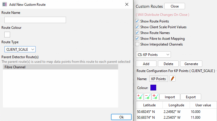
Figure 85: Client Scale

Select OK to create the Client Scale. It is then possible to add, remove and move client scale points on the map. Unique User values must be assigned to each point, and these will be interpolated between pairs of points along the defined route. Checking the 'Show Interpolated Channels' flag will show each client scale channel as a circle along the route. Checking the 'Show Fibre to Asset Mapping' flag will draw lines showing the mapping of each client scale channel to the parent route channel (denoted by the short blue lines in Figure 84).

If coordinates are available in the appropriate CSV format, then these can be imported via the import button. Similarly, a defined client scale can be exported.

When creating a client scale, accurate coordinates must be provided by the client as incorrect points could result in a scale not following the Asset/Fiber Route as intended.

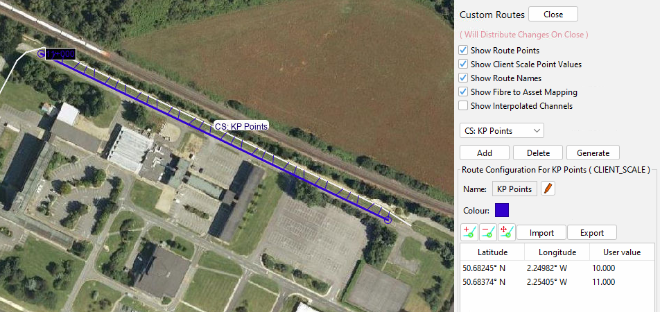
Figure 86: Client Scale with asset mapping enabled

Generating a Client Scale Using Customer Coordinates

In most cases, operators would use the 'Add' button (Figure 85) to create a Client Scale, and import customer-generated coordinate positions. However in some cases the resolution/accuracy of these coordinates may to too poor to follow the required Detector Route as intended. In this scenario, the 'Generate’ option can be used that will generate a Client Scale that will fill any gaps with Detetor Route coordinates between customer-generated coordinates.

To generate a Client Scale using Customer coordinates, press the ‘Generate’ button. This will open a dialogue in which the name, colour and parent Detector Route can be supplied. Ensure that the ‘FromFile’ tab is selected and that the customer CSV file has been selected. The OPS’s this Client Scale should apply to also needs to be selected, and any spurs should be removed from consideration.

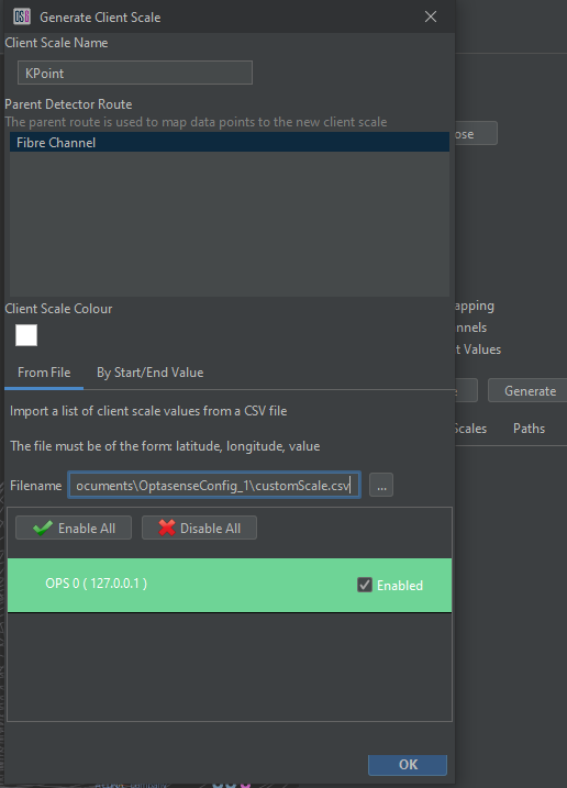
Figure 87: Generate the client scale using customer coordinates

When the OK button is pressed, a Client Scale will be created using a combination of customer and interpolated coordinates with a result similar to Figure 86.

note

A generated scale should be checked to ensure that it provides the expected mapping.

Suppression

There are three suppression methods that can be applied to the system to control how it reacts when faced with the following alert scenario. To access the suppression feature, from the toolbar select Configure and then Suppression.

Figure 89: Detector Suppression

Zone Suppression

A zone can be applied to areas and detector instances turned off where nuisance alerts are being generated by a known signal source. For example, a generator within a secure compound is producing a signal like manual digging. A zone is applied to the area and the manual digging detector instance is turned off. Therefore, no alert will be generated in that area for manual digging activity.

There are 2 ways a zone can be created.

1. From the detector suppression configuration panel, select Add Via Map. A prompt will appear instructing the user to draw an area on the map.
2. The second way is to select Add from the detector suppression configuration panel.

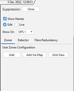
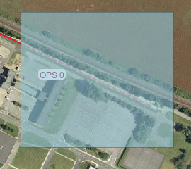
Figure 90: Left - Creating Area Options / Right – Drawing Area on Map.

The next window enables the user to choose what detector instances will be suppressed. By default, all instances will be selected. Deselect any detectors that don't need to be suppressed. Notice below, the channel range, OPS number and colour representing the zone can be edited. Select apply to make the zone active.

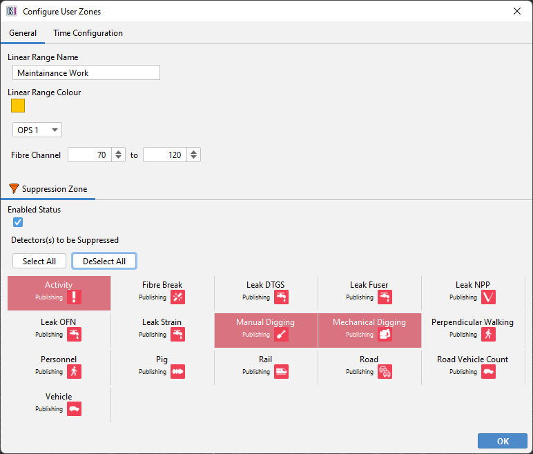
Figure 91: Zone Conditions

Detector Suppression

A detector suppression rule can be applied to allow a generated alert to override (or suppress) other alerts that may be created by the same signal source. For example, a PIG is running through the pipeline and is generating a similar signal source to NPP. Creating a rule where PIG is the suppressor and NPP is the suppressed, means only PIG alerts will be generated.

To create a rule, start by selecting the detector tab from the detector suppression configuration panel. Now select Add.

Figure 92: Add Detector Suppression Rule

There are several options the user can use to aid the configuring of the rule.

The number below explain what can be configured to make up a rule.

1. Select how many OPS the rule is to cover
2. The alert type of the suppressor
3. The alert type(s) to be suppressed
4. The hold time is the amount of time that an alert will be held while the system checks for a suppressor alert. This allows the software time to detect another overarching issue that may be causing the original nuisance alert.
5. Can be used to increase the extent of the suppression area from the start/end channels of the alert or from the alert centre channel.

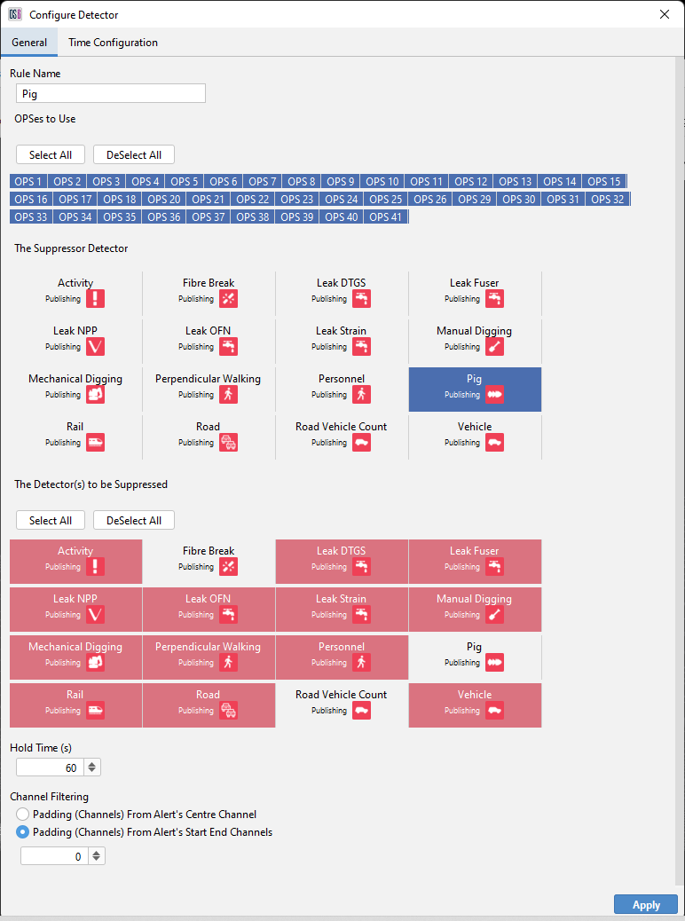
Figure 93: Configuring Detector Suppression Rule

OPS Redundancy Suppression

OPS suppression is used to provide redundancy to two separate OPS's that are covering the same fibre route with one fibre 'suppressing' alerts on the other.

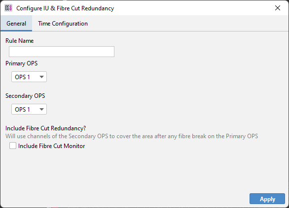
Figure 94: Creating OPS Redundancy Suppression Rule

Suppression Live View

To view live suppression events, they can be observed from the detector suppression configuration panel and map display. To enable this function, select live and toggle the required suppression view or leave as default (Draw All).

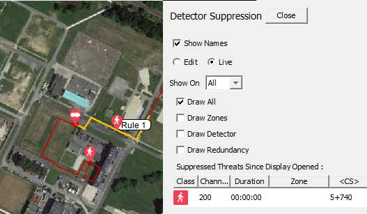
Figure 95: View Suppression Rules

Linear Ranges

It is possible to create a range of channels and associate one or more attributes to it:

1. Suppression
2. Alert Tags
3. Waterfall Frequencies

As per Suppression (see above), a ‘Linear Range’ of Channels can be created and have assigned one or more of the above

Zone Suppression

For details, please see Suppression

Alert Tags

A continuous set of fibre channels can be assigned to have a named ‘Alert Tag’. E.g. when an OptaSense Alert is created within this channel range, it will have the named ‘Alert Tag’ added to the Alert details. This then can be used by a 3rd Party System to identify this location and for example, pan a Camera to this location.

Figure 96: Alert Tag

In the above example, the ‘Entry Gate’ to a perimeter covers Channels 30 to 60. Any Alerts created within these Channels will have ‘Entry Gate’ as the Alert Tag within the Alert Details

Waterfall Frequencies

A continuous set of Fibre channels can be assigned to have user-defined min/max Frequencies. These frequencies do not have any impact on the Detectors. These frequencies only affect the Waterfall display, allowing an Operator to visualize the data for a different set of Frequencies

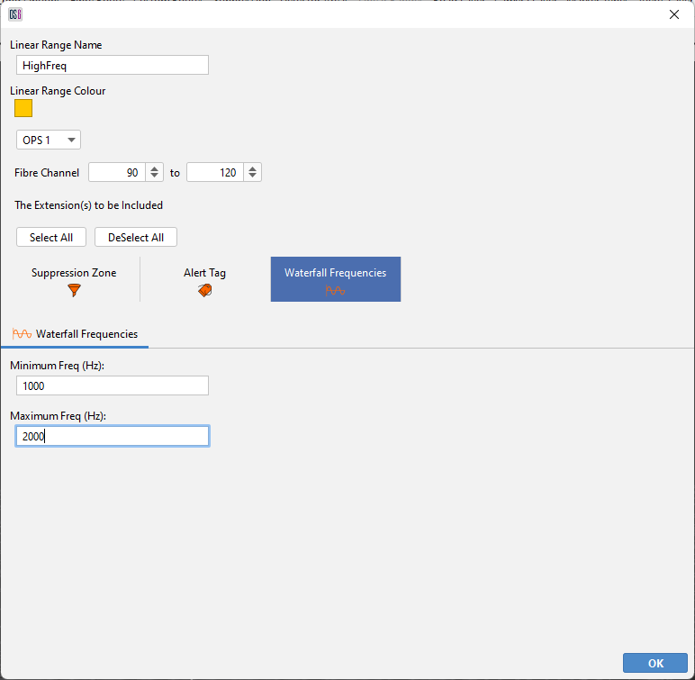
Figure 97: Waterfall Frequencies

Periodic Time Options

Linear ranges can be setup to become active or inactive at certain times/dates using Periodic Times. Periodic Time options are applied per attribute, however only the ‘Zone Suppression’ attribute is supported currently. Below highlights the options available:

Expiry Based Option

Set the attribute to become active/inactive when an expiry time has been reached.

Time Range Based Option

Set the attribute to become active/inactive per day, within a time range (hour/min precision).

Month Based Option

Set the attribute to become active/inactive for certain months out of the year.

Hour Based Option

Set the attribute to become active/inactive for certain hours throughout each day.

Days of The Week Based Option

Set the attribute to become active/inactive for certain days throughout each week.

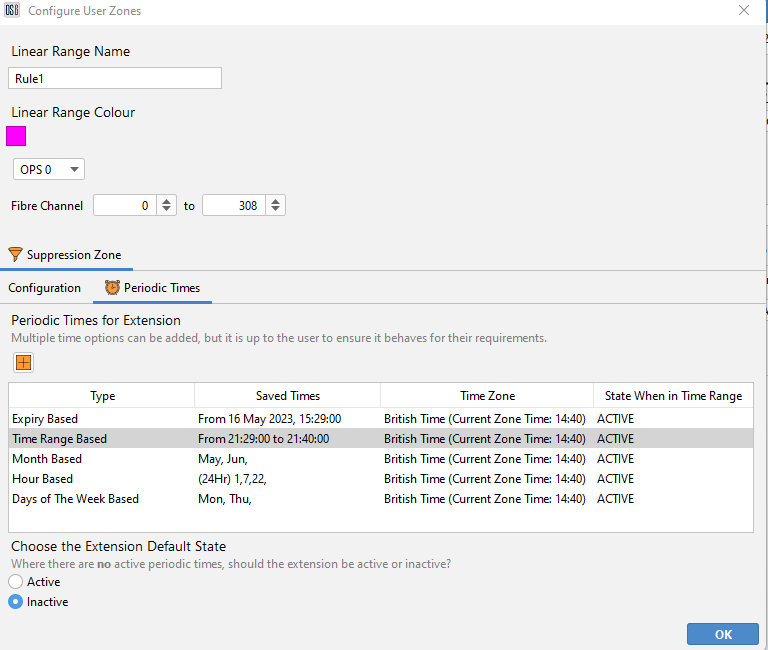
Figure 98: Periodic Times for Suppression Attribute

Multiple Periodic Time options can be added to an attribute (as seen in Figure 98), but it is up to the user to ensure it behaves for their requirements. Periodic Times also do not need to be adjusted for daylight savings.

Area of Interest

The area of interest feature enables the user to view all generated alerts within a specified area and time period. What's useful about this feature is it will display all alerts in a summarised fashion irrespective of whether they were acknowledged or dismissed.

From the toolbar, select Configure and then Area Of Interest. A window will appear to the right of the map display.

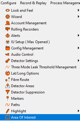
Figure 99: Configuring Area Of Interest

Select Add to choose between drawing the area by channel range or K point. Now draw the required area on the map and when prompted name it appropriately.

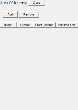
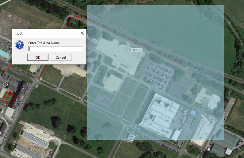
Figure 100: Selecting Map Window

Multiple areas can be created, and their conditions edited at any time. Select Edit to change the following setting.

• Duration: is the amount of days the system will retain alerts.
• Start / End OPS: enable the area to span over two OPS's.
• Remove: will delete a selected area.

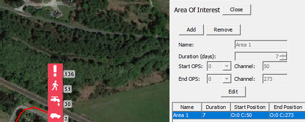
Figure 101: Editing Area

To toggle on and off an Area of Interest showing on the map display, from the toolbar select display and check/uncheck as required.

Figure 102: Toggle Area Of Interest View

Complex Routes

Complex routes allow the user to choose the exact area of fibre they want to apply a zone or suppression area to. This is very useful when dealing with lengths of fibre that pass over each another, loop back on themselves or are connected to separate OPS's. When using complex routes, the software detects the exact OPS channels of the fibre, shown as 'Solution 1' and if possible, offers multiple solutions as seen in Error! Reference source not found..

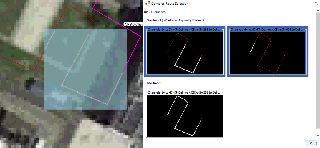
Figure 103: Example complex route solutions

Zoom Areas

A feature added in OS 6.5 is the ability to zoom in user specified areas on the map and display them on the screen at a larger size than their geographical coverage would normally require. This allows, for example a block valve station on a long pipeline to be visible to the operator without having to zoom tightly in on the area, or (as was the only option in earlier versions of the software) having to artificially make the block valve station larger than its actual size in order for it to be visible. This means that alert locations (latitude and longitude) will be correct, where previously with an artificially large area they would not have been correct

Creating a Zoom Area

To create a Zoom Area select the Zoom Area icon from the side bar on the right side of the map window

Figure 104: The Zoom Areas side panel icon

Click the “Add Zoom Area” button and the click and drag on the map in order to create an area around a section of the fibre route to be magnified. Ensure that only the area to be magnified is included.

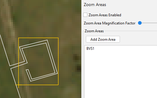
Figure 105: Newly created zoom area

Next, right-click on a location within the newly created area and select “Set Zoom Area Origin” on the point from which the magnification of the area will happen. Everything within the area will be stretched away from this point.

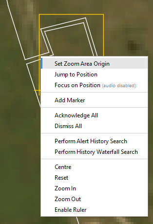
Figure 106: Set zoom area origin

For example on a block valve station, this should be at the point that the fibre leaves and rejoins the pipeline, as shown below

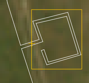
Figure 107: Zoom area origin set as recommended

Finally, the Zoom Area magnification can be enabled and the amount of zoom selected with the sider on the side bar. All items drawn within the area will be zoomed into, this includes the background map image and the size of the blue channel coverage circles.

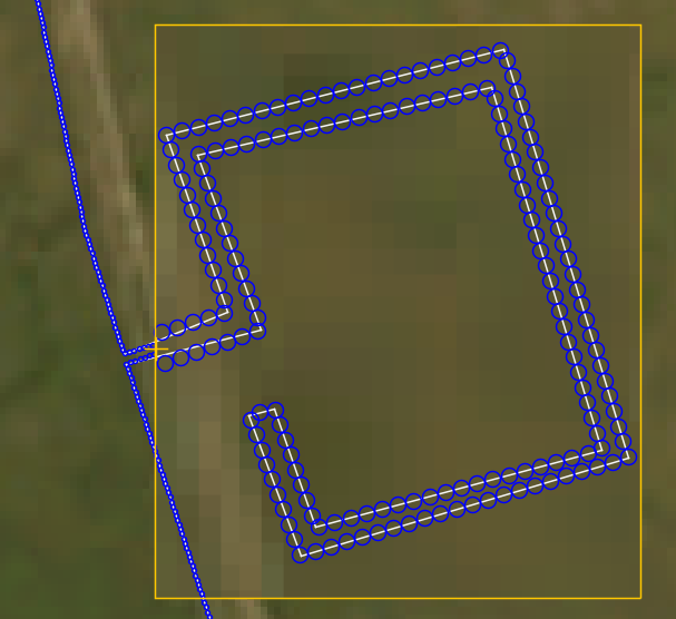
Figure 108: The area zoomed in showing the enlargement of the channel sizes

Final Settings Adjustments

Location and mapping of IU, server and processor nodes logs

All the IU and processor node logs are located on the server node for the system (the PU or DPU). All the information is present in the System Health feature and the logs can be accessed from there.

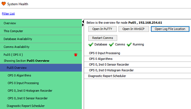
Figure 109: Location of 'Open Log File Location' dialog in System Health

Additionally, this can be accessed via a mapped network drive.

On the CU, open a windows explorer window and select "Map network drive" (displayed on the top toolbar). This will open the "Map Network Drive" window within this window select drive Z and enter the IP address of the server followed by the folder name "logs". The right hand side of Figure 110 shows the log files location opened.

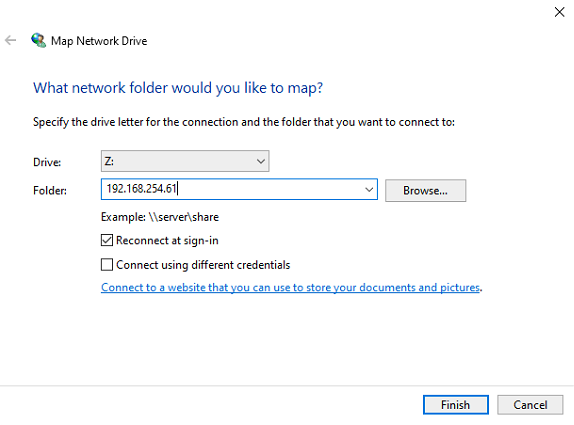
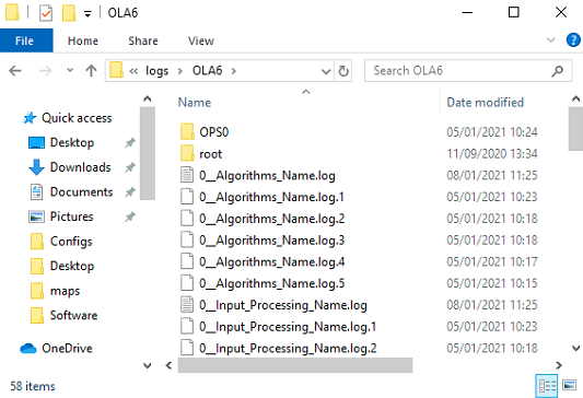
Figure 110: Mapping Network Drive to Server Logs

Location of the CU logs

The CU logs are located on the CU. There is a shortcut to find the location, by left-clicking on the OptaSense software toolbar you can then press F9 and the windows explorer will automatically open at the log location. For information, the full address of the logs is C:\Users\Admin\AppData\Local\OptaSense\OLA6. However, this needs to be typed into the windows explorer toolbar as the folder is hidden so can't be found by just navigating to it.

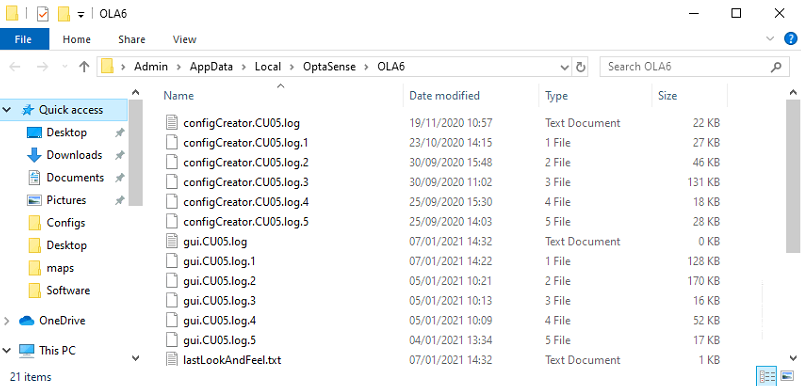
Figure 111: GUI Logs

Location of Windows Background tasks logs

A number of OptaSense tasks are run in the ‘Background’ on the CUs (such tasks to to do with re-sizing the System). The location of these logs are on the specific CU

C:\Windows\System32\config\systemprofile\AppData\Local\OptaSense\OLA6

Location of Database logs

The logs associated with the Cassandra Database can be found on the Processing Units, as each PU has an instance of Cassandra running on it. To access/view these logs, it is recommended to use ‘putty’ or ‘WinSCP’. The location is:

/var/log/cassandra/system.log

The Homepage

Numerous hardware items within the OptaSense system have web interfaces which enable a lot of configuration changes to be made. All of these are linked to a homepage that is custom-built for each project.

The pieces of equipment that are linked through the homepage are:

• All server and processor nodes (PS, DPS, PU and DPUs) have the IPMI enabled.
• All desk mounted Netgear switches
• All ECPSs
• Dry contact moxas
• SDS for any SMS facility.

Figure 112: OptaSense CU Homepage

Control Unit - shared modification record.

Each CU should also have access to the modification record. To do this:

• Add another folder on the C: Drive of the primary CU entitled the 'Modification record'. Add the modification record from huddle.
• On each CU, create a shortcut on the desktop entitled 'Modification record' and point the CU to the correct location of the 'Modification record' folder on the primary CU

Setting up the Fibre route

The fibre route details that are supplied by the customer need to separate per OPS and placed in a .csv file. This can be achieved via Microsoft Excel, two columns need to be populated, the left for the Latitude values and the right for the longitude values. Once one file has been created for each OPS this needs to be saved as CSV files.

Figure 113: Lat/Long CSV file

To import these values into the OptaSense software the following instructions need to be followed:

1. Open the OptaSense software
2. Open a Map display
3. Select Configure – Fibre Layer
4. Click on Edit Installation. Click OK to acknowledge the warning about switching of the algorithms.

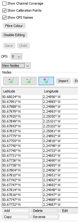
Figure 114: Edit Fibre Route Installation

1. Select OPS 0 from the OPS drop down box
2. Click on import, then locate the .csv file saved with the OPS 0 Lat/Long positions
3. Ensure "File contains Lat/Long coordinates" and click OK within the "Select CSV File Type"
4. Select "Save" to save the changes
5. Follow steps 5-8 for all other OPS'

Advanced GUI Tools

Surveillance Waterfall

The surveillance waterfall enables users to view live acoustic sensor data in graphical format. Activities, as they occur, can be observed through the display, and tools can be used to analyse their source in better detail. To access the waterfall, from the toolbar, select Live Analysis and then Waterfall.

Figure 115: Opening Surveillance Waterfall

Waterfall Options

There are several options that can be used to customise the appearance or aid analysis using the waterfall. As shown in Figure 116::

1. OPS – OPS Waterfall Selection
2. X-Axis – Allows the X-axis scale to be changed to a configured Client Scale or Detector Route
3. Scaling – Changes the Histogram scaling and colour values
4. General –
   • Use Whitened Source – switches between regular and whitened waterfalls
   • Track Alerts on Waterfall – determines whether alerts are tracked on the waterfall
   • Change Default Frequency Band – Allows the waterfall frequency band to be altered
5. Right Click on Waterfall - Allows access to rate, interrogation options and mouse mode options (speed check, creating areas/zones)

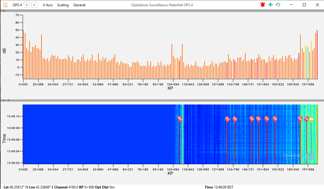
Figure 116: Waterfall Options

Waterfall Frequencies

Another feature of the waterfall display window is the ability to display specific frequency bands. Note that this frequency band selection does not affect the frequencies utilised within the detectors, nor will it modify the sensitivity of the system. This will, however, modify the histogram data when viewed on the waterfall in addition to any subsequent histogram rolling recorder files.

The frequency band used for the waterfall display can be altered by selecting General> Change Default Frequency Band from the drop-down bar at the top of the waterfall. This will open the dialogue box, as shown in Figure 106.

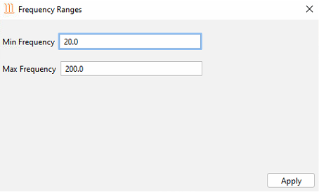
Figure 117: Waterfall Frequency Ranges dialogue box

The default frequency range for the waterfall display is 20 to 200 Hz. This can be tailored on each system to help identify different events.

Live Frequency Analysis window

The Frequency Analysis window enables the user to carry out frequency analysis on the live waterfall. To access this feature, from the toolbar select Live Analysis and then Frequency analysis.

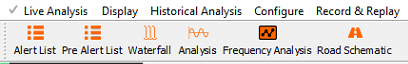
Figure 118: Opening Frequency Analysis Window

The frequency analysis panel displays fibre channels in the x-axis and frequency in the y axis.

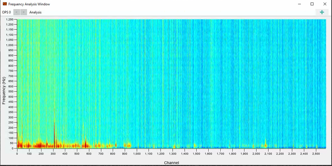
Figure 119: OPS Frequency Analysis Window

Using the menu bar options, the user can change the selection of OPS data to display and by opening the Analysis>Settings dialogue (Error! Reference source not found.) the colour scaling and the decay rate of the data can be changed.

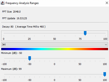
Figure 120: Frequency Range Adjustment

Record and Replay

Record & Replay enables live sensor data to be recorded and replayed later. Note, only trained user accounts have access to this feature. From the toolbar, select Record & Replay.

Figure 121: Selecting Record & Replay

Recording

From the main Record & Replay menu, select the required OPS (top left), then Start New Recording. Fill out the required details, for example, the activity and channel number (Man Dig CH2000). Selecting OK will start the recording. To stop it, right-click on the running recording and select stop.

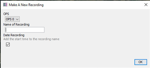
Figure 122: Record/Replay Window

While recording, if an event of interest occurs, notes can be added to the recording to mark the event. Right-click on the recording and select Add Event. Fill out the text field with the required details and select OK.

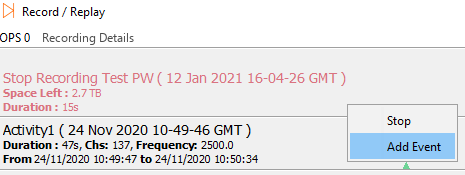
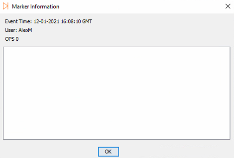
Figure 123: Left – Add Event to Recording / Right – Giving Event Description

Replay

To replay a recording, whilst in the Record & Replay window, right-click of the required recording and select Play. (NB Replaying a recording will prevent the processing of live data. Similarly, the rolling recorder processes will record the replaying data). A window will appear where the user can alter the replay parameters:

• Loop – Automatically replay the recording once it's finished
• Play With Current Time – Plays the recording as if it were in real current time. Unchecking it will replay the recording with its original time/date
• Start / End Fields – Enables the start and end time to be edited, which is useful for skipping to certain parts of a recording.

When a replay is running, events can be added by rightclicking on the recording in replay and selecting ‘Add Event’.

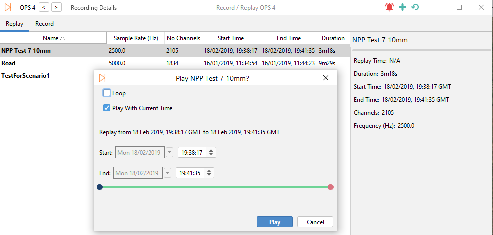
Figure 124: Left – Play Recording / Right – Recording Replay Properties

Manual Record Path

The manual record path, by default, is set to the following location /mnt/disk4/ManualRecord0. This shouldn't need changing; however, it can be done so by selecting Recording Details and then Change Record Path whilst in the Record & Replay window.

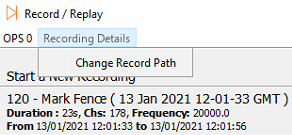
Figure 125: Change Record Path

System Area Lockdown

There are certain areas within the system that are locked down to prevent unwanted changes being made to them. Only those with SuperUser Access can enter a code and unlock them.

Time-Based One-Time Password (Access Code)

In order to elevate to a superuser, an access code will need to be entered when logging into the system. To do this, launch the software and at the login page check Log In As Super User.

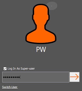
Figure 126: Entering Password

The window will change and ask the user to enter a one-time code. For information in relation to obtaining the code, refer to the next section.

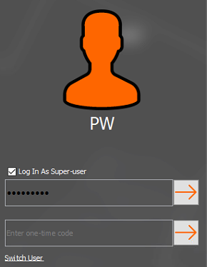
Figure 127: Entering One-time Code

Forgotten Password (Superuser)

In the case a superuser cannot remember their password, the password can be reset. This can be done from the login page by using the ‘Forgot Password’ link. This link is only available for superusers. If non-superusers have forgotten their password, a superuser would need to reset it in the Account Management display.

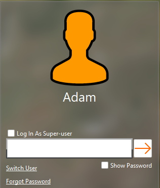
Figure 128: Forgot Password Link

When resetting the superuser password, the One-Time Password (Access Code) will need to be entered in along with the new password.

Figure 129: Forgot Password Display

If a valid One-Time Password (Access Code/TOTP) is entered along with a valid password that conforms to the complexty requirements, the password will reset.

OptaSense Authorisation Server

Firstly, the user will need to access the OptaSense Authorisation Server. This can be done using any typical internet browser.

In the search bar, enter the following address: https://auth.optasense.com

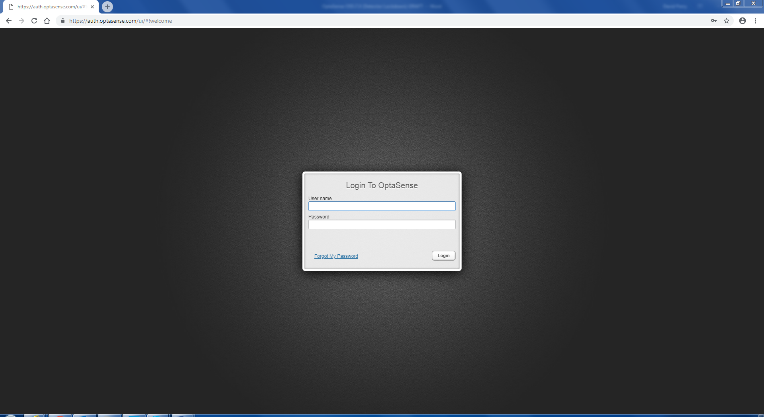
Figure 130: Authorisation Server Log In

Each user will have log in details that will give them access to the server.

Once the correct login details have been entered, they will be taken to the main homepage of the authorisation server.

Figure 131: Authorisation Server Homepage

In the top left of the screen, click on the menu drop down box and select Groups.

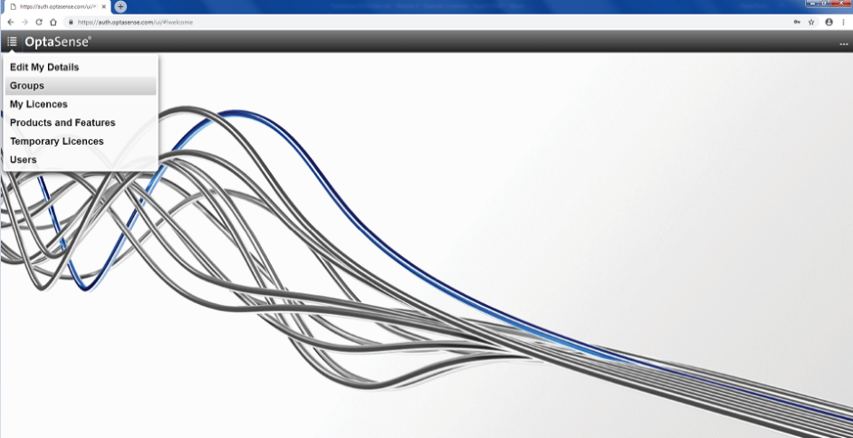
Figure 132: Group Selection

A software licence must have already been created. The generated access code links to the MAC address of the system that requires access. An access code generated using a different licence group will not work. The created licence can then be found and selected within the Groups drop-down window.

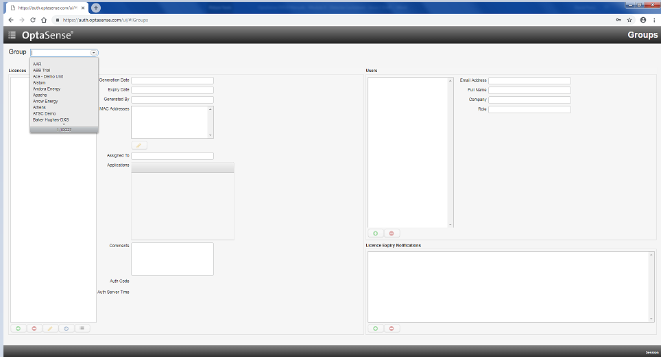
Figure 133: Dropdown Window Group Licence Selection

Having selected the appropriate group from the list, the authorisation server will now display the different licences that relate to the project system. Some systems may have multiple licences attached to their group. This is dependent on the number of CUs within the system.

Selecting the appropriate licence provides the user with an Auth Code. This is the code that needs to be entered as the one-time code. As stated, the access code will regenerate every 30 seconds. A countdown timer, as well as the current Authorisation Server time in UTC, will be displayed. The time displayed allows the user to make a comparison between the server and the CU being worked on. Once the timer has reached zero, the code displayed will expire and a new code will be generated. The code must be entered within 10 minutes of generation.

Once the access code has been entered, the user will now have full system access.

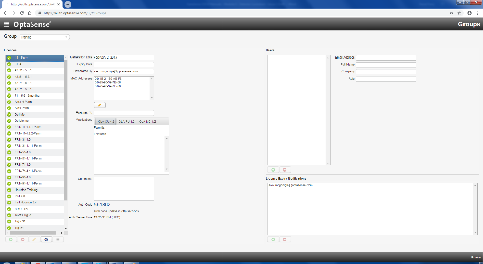
Figure 134: Generated Access Code

Contacting an Authorised OptaSense Engineer

If a user requires Super User access and they do not have access to the OptaSense Authorisation Server due to the lack of a reliable internet connection, then it will be necessary to contact an authorised person from OptaSense or to arrange a support contract that includes code access.

Once in contact with an authorised person, the onsite user will need to provide details of the project so that the correct Group and Licence can be found.

Detector guidance for local administrators

As a Trained User, it is possible to modify the detector settings. The detectors are configured during the initial commissioning and SAT stages of installation in line with the clients' Threat Profile. The detectors are updated during IOC-FOC improving the overall alert rate and reducing nuisance alerts. Note that the sensitivity of the system is dependent on environmental factors such as ground types and seasonal variations.

Fibre Break Detector

The fibre break detector implements one of two potential fibre break detectors dependent on the IU version. If the IU in use is an OLA 2.1, then the 'Fiber Break Old' detector window will be available.

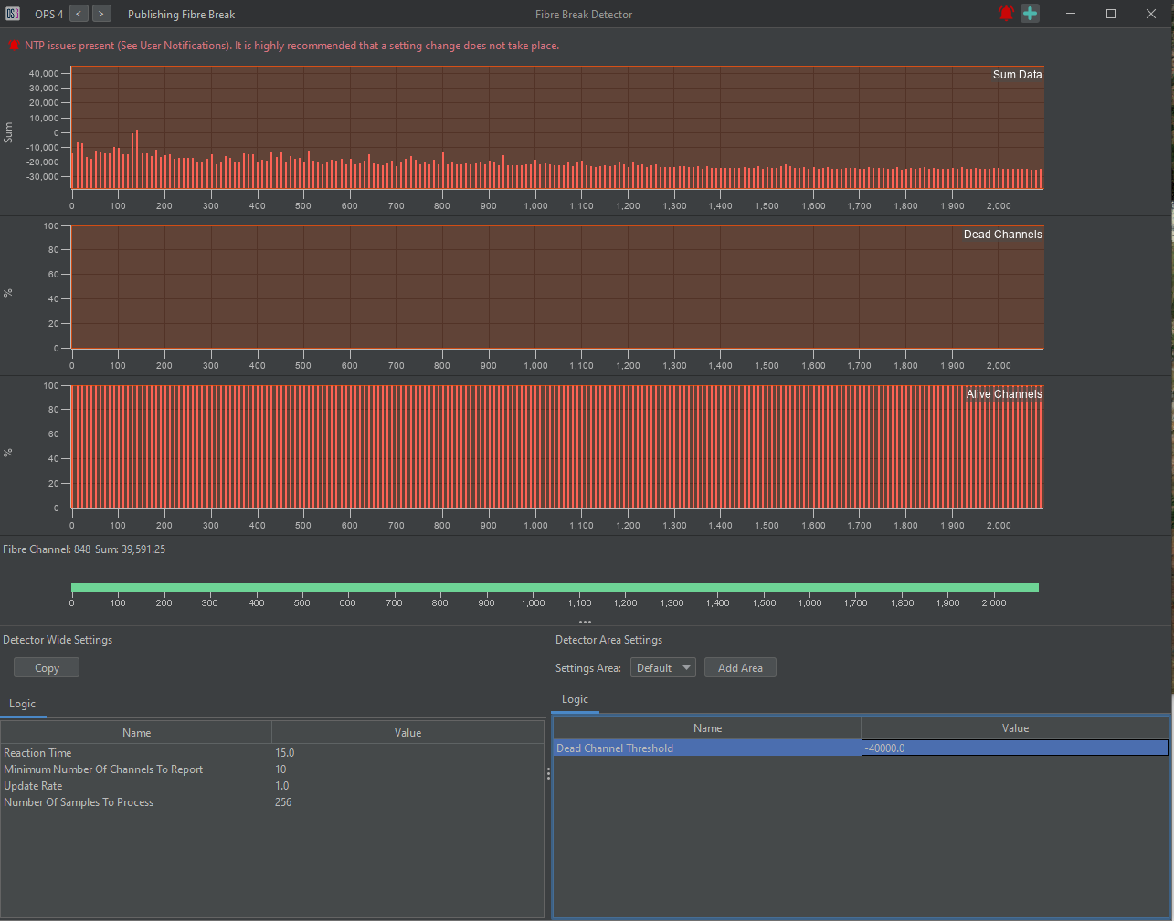
Figure 135: Fibre Break Old Detector Panel

As with previous versions, fibre break is configured by entering a threshold value based on the lowest value shown in the detector window and then selecting the number of consecutive channels required to drop below this value before an alert is published.

If the IU version is 2.1+ or QuantX, then the IU assurance stream will manage the fibre break detector and should be set up automatically as long as assurance is enabled within IUSetup. The assurance stream requires no further configuration.

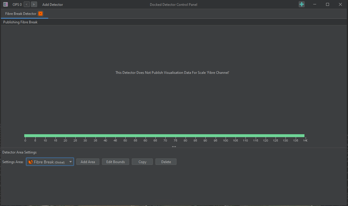
Figure 136: Fibre Break with IU Assurance stream

If the assurance stream or processing is not on, a user notification is flagged, and an error will be published.

Activity Detector

The activity detector is a very flexible detector and is used for a wide range of different threat events. It works by locating channels which have a noise signature above their historical values. This signature is tailored in many ways to the event, such as in intensity, frequency and duration.

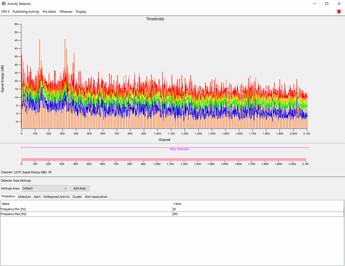
Figure 137: Activity Detector

Personnel Detector

The personnel detector is used to detect parallel walking near to a given asset. It comprises a detection element, which first locates step-like impacts, before handing these events into a tracking element. The tracking element is used to confirm that velocity associated with walking appears in these impacts before triggering an alert.

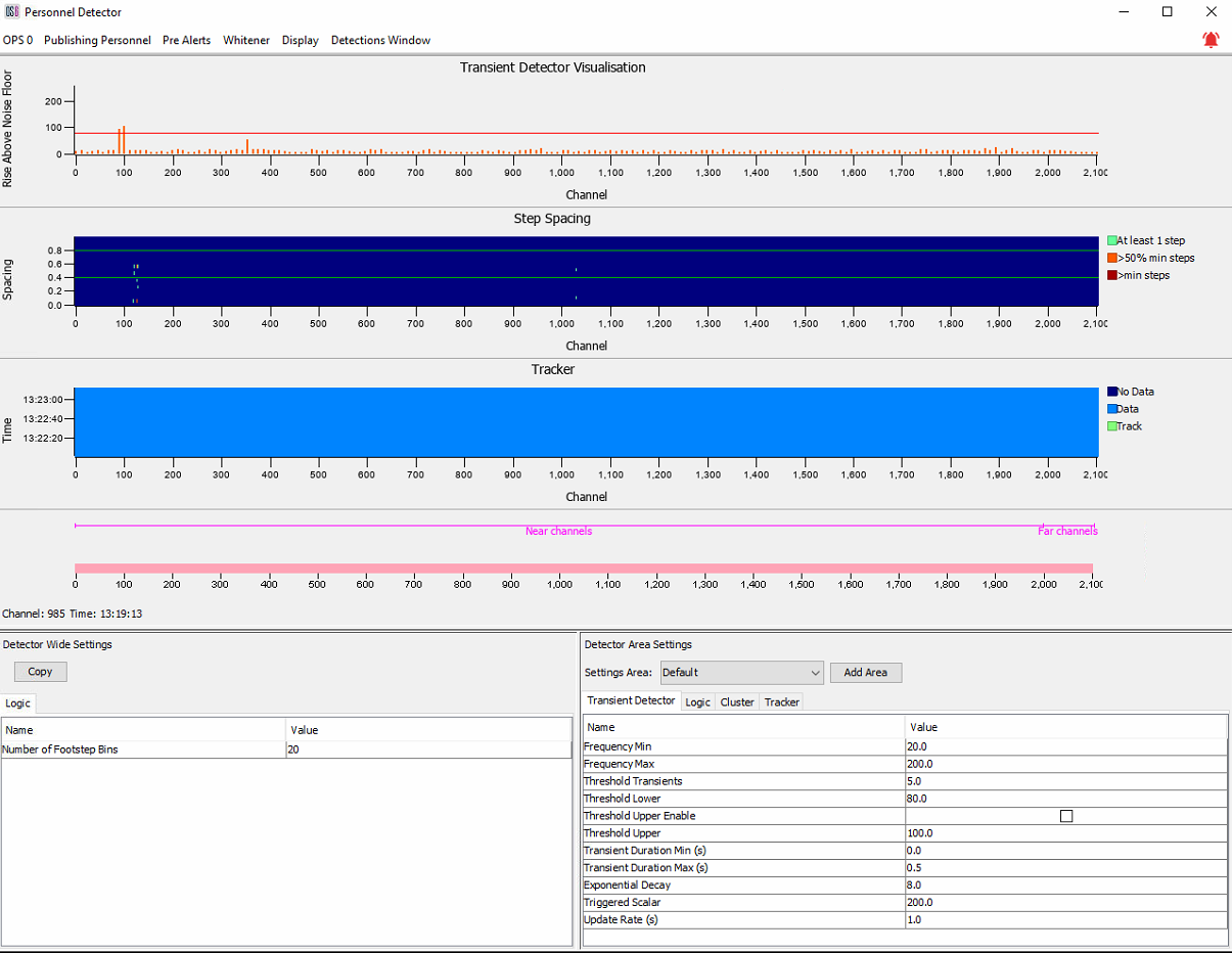
Figure 138: Personnel Detector

Vehicle Detector

The vehicle detector is used to detect individual vehicles progressing parallel to the fibre. It searches for events which are louder than the noise floor by a pre-determined level before tracking these events to ensure they move in a way expected by vehicles, at which point an alert would be raised.

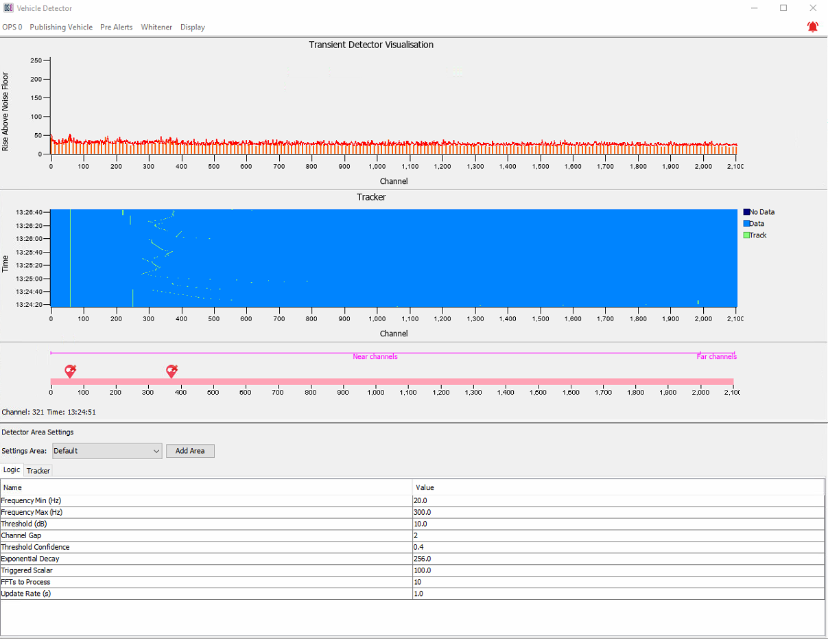
Figure 139: Vehicle Detector

Manual Digging Detector

The manual digging detector captures individual, short impact-like events and tracks the repetitive frequency and pattern of these events. If the impact events satisfy several criteria associated with manual digging, an alert will be raised.

Trained Users can modify the detector logic to fine-tune the detector.

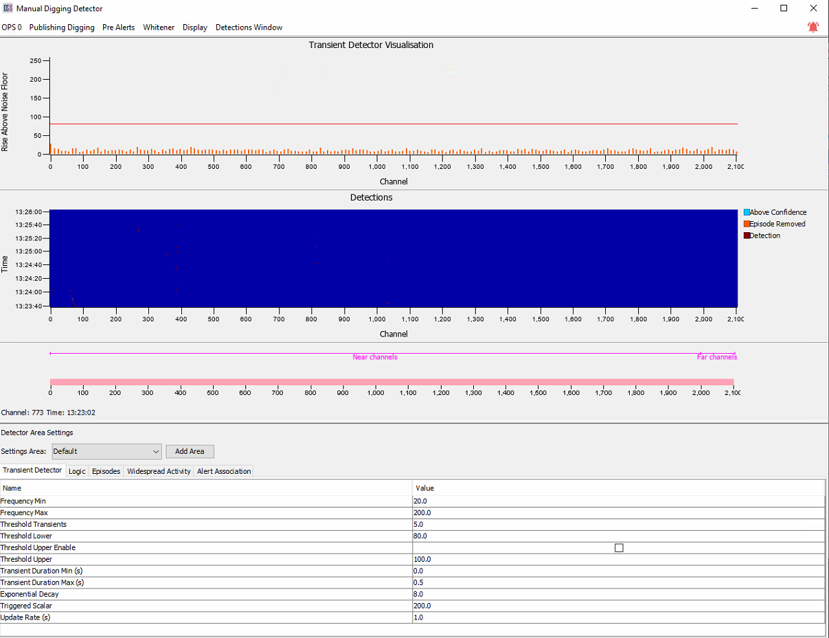
Figure 140: Manual Digging Detector

Mechanical Digging Detector

The mechanical digging detector works in a similar way to the manual digging detector by capturing individual, short impact-like events and tracking the repetitive frequency and pattern of these events. However, it differs with the addition of a tonal detection element; tonals result from running engines and can be used to add confidence to a detection before an alert is raised.

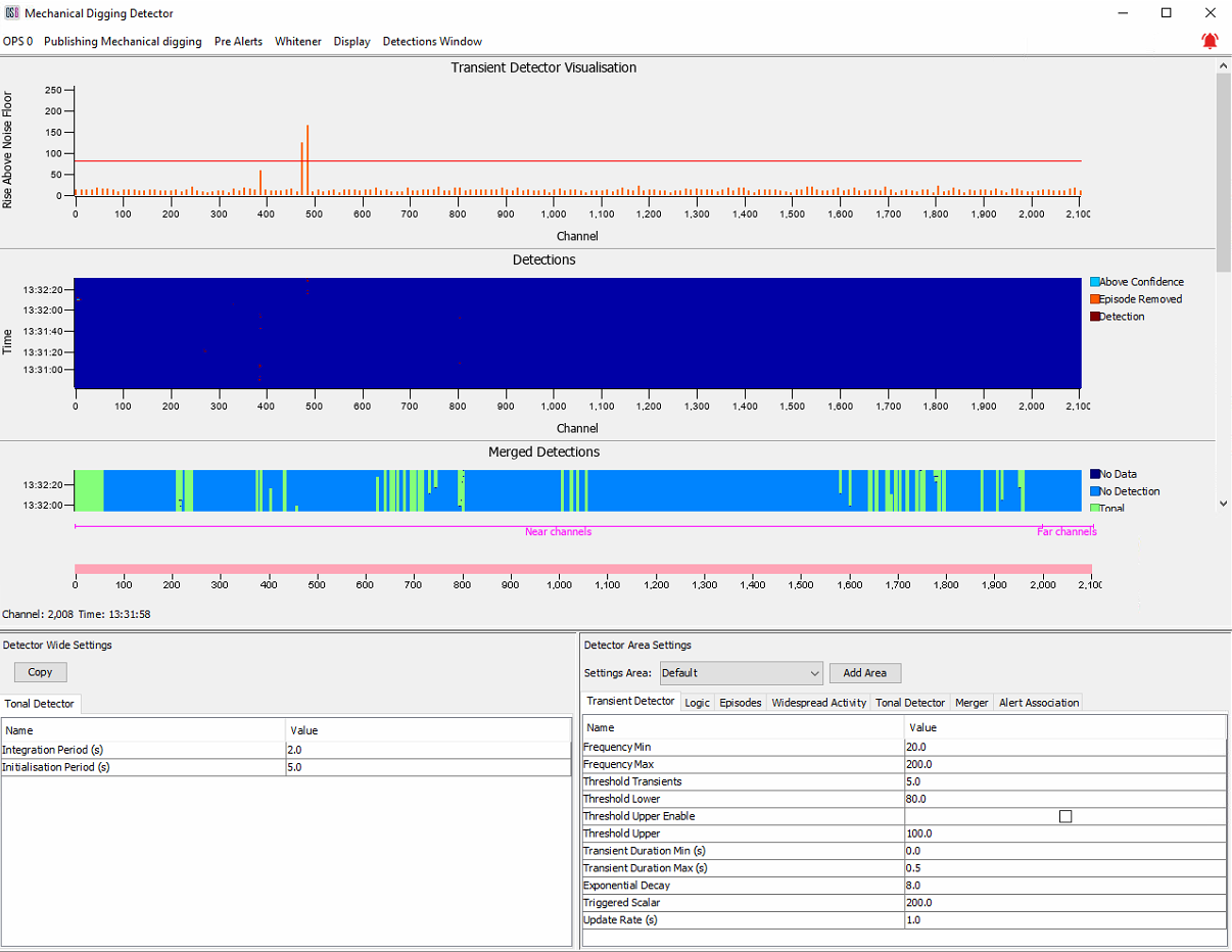
Figure 141: Mechanical Digging Detector

PIG Detector

The PIG detector is used to detect and track the movement of pigs within pipeline assets. It does this by detecting the characteristic pressure pulses that are transmitted by pigs as they progress through the pipeline. The PIG detector panel does not display any information.

Sensor Whitener

The Sensor Data Whitener is an algorithm which suppresses high levels of constant background noise in the input time series data received from the DC filter. It does this by flattening and levelling the spectrum of the signal through an adaptive spectral whitening filter. After whitening, transient events in the signal with different spectra from the background noise are emphasised, and both the waterfall clarity and the detector/classifier performance are improved

The following two images show the removal (or whitening) of constant noise. The first image is from a scenario without an active whitener, and the second shows how an active whitener in the same scenario quickly 'learns' of the continuous background noise and removes it.

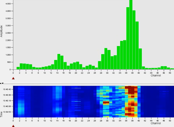
Figure 142: Unwhitened Waterfall

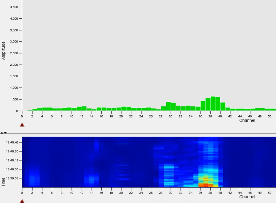
Figure 143: Whitened Waterfall

Processing Chain

The Sensor Data Whitener operates early in the data processing chain after the sensor data has been DC filtered. Some detectors can be configured to use whitened or unwhitened data. The whitener must be used carefully with data to be processed by detector/classifiers looking at long-duration signals. Detectors looking for tonal signals - such as from engines - look for long-duration signals that can be dampened by the whitener.

Observing the Whitened Stream

By default, the waterfall will connect to the unwhitened data stream. The waterfall display can be configured to connect to the whitened data stream by checking the "Use Whitened Source" option in the "General" menu. This will not impact any detectors.

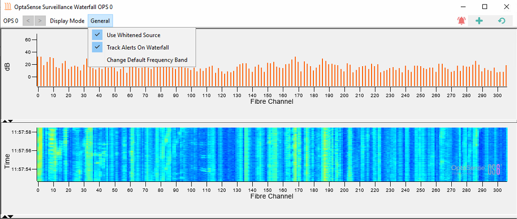
Figure 144: Waterfall display showing how to enable the whitened data stream

Detectors Control GUI

The OptaSense Detector Control Window contains a number of pages to assist in configuring each detector instance. Where applicable, these pages contain a checkbox to connect the detector instance to take the whitened chain as its input for FFT and histogram data. Toggle this checkbox on to connect to the whitened chain rather than to the non-whitened DC-filtered only chain.

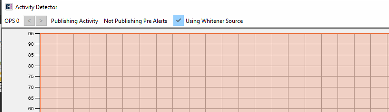
Figure 145: Activity DCP with whitened data stream flag enabled

The results of the detectors' processing of the whitened data can now be observed on the OptaSense Detector Control Window page displays.

Glossary of Useful Commands

Linux (Putty)

Command	Description
systemctl stop <process>	Stops the named process. See table below for processes and descriptions
systemctl start <process>	Starts the named process
systemctl restart <process>	Restarts the named process
ps -ax | grep java	Check running java processes
ifconfig | more	Check IP addresses, etc
cd	Change directory
ls	List files in current directory
unalias ls	Makes the stuff in the directory easy to read
ls -l	Puts it in a list
cd ..	Moves back up a directory
xx -help	Displays help for 'xx'
reboot	Reboots server
df	Displays disk information
du	Displays directory usage information
date	Displays current date
uptime	Tells you how long server has been running
pwd	Displays current directory path
more <file>	Reads out contents of file
cp -r *.* /mnt/..	Copies contents of directory to new location
mv -r	Moves directories or files
<up arrow>	Brings up previous commands
<tab>	Auto completes filenames, directories, etc.
ping xxx.xxx.xxx.xxx	Pings IP address
rm -rf -v 'directory to delete'	Deletes files and directories
-r	Recursive - directory and everything below it
-v	Verbose - lets you know what the command is doing
:q	Quit vi
:q!	Force quit vi
:qw	Quit and write in vi
su root	Changes user to root
ssh root@xxx.xxx.xxx.xxx	SSH into a node
top -n 10 -b > /mnt/../abc.txt	Runs "top" in batch mode and creates a .txt file with 10 updates of the real-time "top" information.
top Then type "1" Then type W	This makes the top command run showing CPU usage for each core by default. The command above (top -n 10 -b > /mnt/../abc.txt) can then be entered Runs "top" in batch mode and creates a .txt file with 10 updates of the real-time "top" information. To create a .txt file including the individual CPU core information.

Process Name	Description
optasense-user.target	Target combining all OptaSense user processes (Input Processing, Algorithms, Rolling recorders, etc)
dummyHazelcast	Hazelcast cluster member process
cassandra	Cassandra Database

Windows (cmd)

Command	Description
ping xxx.xxx.xxx.xxx	Pings IP address 4 times
ping xxx.xxx.xxx.xxx -t	Pings IP address indefinitely
w32tm /query /configuration	Display Windows NTP configuration

OptaSense Support Portal

OptaSense offers various options when it comes to supporting systems in operation. Most common is remote support, however, occasionally, onsite support visits are requested, and an OptaSense Engineer will visit the site and remedy any problems. If you have a support contract and would like to raise a request, you can contact us at http://support.optasense.com

For enquiries regarding obtaining a support contract, please also use the address above.